14.3 Multiple Regression
Here’s a thought experiment. In which scenario could one more accurately predict a student’s GPA?
Knowing how many hours the student spends on schoolwork each week
Knowing how many hours the student spends on schoolwork each week plus his or her high school GPA, his or her IQ, and how much alcohol the student consumes each week
Most people believe the additional information in Scenario B is relevant to predicting academic performance and they are correct. In Scenario B, the prediction should be more accurate because more factors are taken into account.
556
The difference between Scenario A and Scenario B is the difference between simple regression and multiple regression. The previous section focused on simple linear regression. Simple regression uses just one predictor variable to calculate Y′. Multiple regression uses several predictor variables to calculate Y′. If the different X variables have different influences on the outcome variable being predicted, when they are combined, they will do a better job of prediction than any one variable by itself.
r2, the percentage of variability in the outcome variable that is accounted for by the predictor variable(s), is called R2 in multiple regression. Better prediction means a higher percentage of variability is accounted for with multiple regression than with simple regression. In this way, multiple regression is a more powerful technique than simple regression.
Deriving a multiple regression equation is beyond the scope of this text. But, here is an example to show how it works. Every year, colleges have many more applicants than they can admit. Part of the admissions process involves deciding which applicants can do college-level work. Multiple regression plays a role in predicting which applicants will fare well in college.
The College Board, the folks who created the SAT, provide a service to colleges that it calls ACES, the Admitted Class Evaluation Service. ACES uses admissions information from a first-year class to develop a multiple regression equation to predict first-year GPA. Once this equation is developed, the college can apply it in subsequent years to applicants to predict what their GPAs will be. The college can decide whom to admit, objectively, on the basis of predicted GPA.
The College Board offers a sample ACES report on its website (collegeboard.com). Using hypothetical data, the Board examines how well four variables—SAT reading subtest scores, SAT writing subtest scores, SAT math subtest scores, and high school class rank—predict first-year GPA for about a thousand students at one college.* [High school class rank is transformed to range from 100 (the best student) to 0 (the worst student).] Here are the Pearson r correlation coefficients for each of these variables predicting GPA by itself:
* Note: This example is based on the three-section SAT in use prior to 2016. Beginning March 2016, the SAT includes only two sections, Reading/Writing and Math.
SAT reading test, r = .42
SAT writing test, r = .42
SAT math test, r = .39
High school class rank, r = .52
These r’s are all fairly close to each other in terms of size. The r with the strongest correlation with GPA, meaning the one that is the strongest predictor, is high school class rank. There is certainly some overlap in what these four variables measure and how well they predict GPA. For example, general intelligence level plays a role in all four scores and intelligence plays a role in determining GPA. But, each of the four variables also measures something unique. For example, part of how well one does on the math test is not a result of one’s general level of intelligence or the reading and writing skills that help on any test. But, to some degree, performance on a math test is determined by specialized math skills. And, to some degree, these same specialized math skills play a role in some of the courses that determine the GPA. Multiple regression adds together the unique predictive power of each variable. As a result, multiple regression usually accounts for a bigger percentage of the variability in the outcome variable than is accounted for by any single variable.
557
When the four College Board variables are combined together to predict GPA in a multiple regression, the correlation climbs to R = .57. (The abbreviation for the correlation coefficient for multiple regression is R, not r.) This doesn’t sound like much of an increase from the .52 correlation between class rank and GPA. But, it is. The percentage of variance explained changes from 27.04% to 32.49%. Predicting an extra 5 percentage points of variability is very worthwhile.
The multiple regression equation the College Board develops for a college can be used to predict GPA from SAT scores and high school rank for a potential student. Their equation is a more complex version of the linear regression equation from earlier in this chapter. The equation has “weights” for each of the predictor variables. The weights are like the slope in the linear regression equation. And there is a constant that is like the Y-intercept. When all of this information is put together, it makes for a long equation. Here is how estimated GPA, GPA′, would be calculated:
GPA′ = (SATReadingScore × WeightReadingScore) + (SATWritingScore × WeightWritingScore) + (SATMathScore × WeightMathScore) + (HSRank × WeightHSRank) + Constant
Here are the four weights and the constant for the College Board example:
Reading weight = 0.0012
Writing weight = 0.0013
Math weight = 0.0006
HS rank weight = 0.0029
Constant = 0.7821
If an applicant were good at reading (SAT score = 600), not so good at writing (SAT score = 450), very good at math (SAT score = 760), and had a very good class rank (90), then her predicted GPA would be
GPA′ = (SATReadingScore × WeightReadingScore) + (SATWritingScore × WeightWritingScore) + (SATMathScore × WeightMathScore) + (HSRank × WeightHSRank) + Constant
= (600 × 0.0012) + (450 × 0.0013) + (760 × 0.0006) + (90 × 0.0029) + 0.7821 = 0.7200 + 0.5850 + 0.4560 + 0.2610 + 0.7821 = 2.8041 = 2.80
A person with those SAT scores and class rank would be predicted to end up with a GPA of 2.80 at the end of her first year.
The multiple regression equation is built from cases where the first-year GPA is known. The equation can be used to predict first-year GPA for these students. As a result, the students have both actual and predicted GPAs, and it is possible to see how well the predicted GPA predicts the actual GPA. The correlation between the two is .46. Multiple regression makes objective predictions that minimize errors in prediction overall. In that sense, it makes better decisions. But, unless R = 1.00, it doesn’t make perfect predictions.
Worked Example 14.3
Many Americans are trying to lose weight, either by counting calories or by using Weight Watchers®. One of the two Weight Watchers plans counts points, not calories. In its system, foods are assigned a point value based on a mysterious combination of how much protein, carbohydrates, fat, and fiber the food contains. The number of calories in the food is not part of the equation. With the point system, a cup of lettuce is worth 0.3 points and a McDonald’s Quarter Pounder is worth 13.4 points.
558
Imagine that a nutritionist, Dr. Feldman, wanted to crack the secret equation that Weight Watchers uses and figure out how these four variables—protein, carbs, fat, and fiber—are combined to generate a point score. This calls for multiple regression.
First, Dr. Feldman draws a random sample of foods and for each one he finds out how much protein, carbs, fat, and fiber the food contains. He also consults the Weight Watchers Web site and locates the point value for each food. Armed with these four predictor variables (protein, carbs, fat, and fiber) and the one outcome variable (points), he uses SPSS to find the multiple regression equation. The equation that calculates Points′, the estimated number of points, is
Points′ = (GramsProtein × WeightProtein) + (GramsCarbs × WeightCarbs) + (GramsFat × WeightFat) + (GramsFiber × WeightFiber) + Constant
= (GramsProtein × 0.074) + (GramsCarbs × 0.096) + (GramsFat × 0.279) + (GramsFiber ×
–0.101) + 0.112
Note that three of the weights are positive, but the weight for fiber is negative. This reveals that fiber plays a different role in determining points than do the other three variables. As the levels of proteins, carbohydrates, and fats in a food go up, so does the point value for the food. However, as the amount of fiber in a food goes up, the point value goes down.
An important use of a regression equation is to predict a value for a new case. Suppose Dr. Feldman is about to eat a BLT and wants to know how many points it is worth. From the menu, he learns that the sandwich has 15 grams of protein, 28 grams of carbohydrates, 17 grams of fat, and 3 grams of fiber. Here’s how he would calculate its points:
Points BLT′ = (GramsProtein × 0.074) + (GramsCarbs × 0.096) + (GramsFat × 0.279) + (GramsFiber × –0.101) + 0.112 = (15 × 0.074) + (28 × 0.096) + (17 × 0.279) + (3 × –0.101) + 0.112
= 1.1100 + 2.6880 + 4.7430 – 0.3030 + 0.112 = 8.3500 = 8.35
Dr. Feldman has now estimated (predicted) that eating a BLT at lunch will use up 8.35 of a person’s daily point allowance.
Practice Problems 14.3
Review Your Knowledge
14.08 Explain why multiple regression explains a larger percentage of variability in the predicted variable than does simple regression.
Apply Your Knowledge
14.09 A multiple regression equation has a constant of 55.12, a weight of 13.17 for variable 1, and a weight of 4.55 for variable 2. If a case has a score of 12 on variable 1 and a score of 33 on variable 2, what is Y′?
559
Application Demonstration
Let’s see multiple regression in action. In this cost-conscious era, hospitals try to save money by reducing the length of stay of their patients. It would be beneficial to a hospital if it could predict a patient’s length of stay at the time of admission. If so, therapeutic resources could be directed to the patients predicted to be in the hospital for a long time, in order to help them get better more quickly.
Some researchers turned their attention to predicting length of stay for patients admitted to a large, metropolitan psychiatric hospital (Huntley, Cho, Christman, & Csernansky, 1998). In a six-month period, almost 800 patients were admitted to the facility and they spent an average of 16.3 days in the hospital. The hospital database contained a lot of information about each patient, including each patient’s sex, age, primary and secondary diagnoses, number of prior admissions, and legal status. The researchers combined these variables using multiple regression to see if length of stay could be predicted.
There turned out to be five variables that played a statistically significant role in predicting a patient’s length of stay: (1) a primary diagnosis of schizophrenia, (2) the number of previous admissions, (3) a primary diagnosis of a mood disorder, (4) age, and (5) an alcohol or drug problem as a secondary diagnosis. These variables can be thought of as reflecting difficult cases. For example, someone with five previous psychiatric admissions probably has a more severe problem, one that may take longer to treat, than a patient for whom this admission is the first hospitalization.
Together, these five variables predicted 17% of the variance in length of stay. This may not sound like much, but Cohen (1988) would call it a medium effect. Is it enough to be useful?
So far, what these researchers did is not unusual. But, now their work took an interesting direction. They used their regression equation to calculate the predicted length of stay for each patient. As a result, there were two pieces of data for each patient—the actual length of stay and the predicted length of stay. The researchers then added a third variable for each patient—the psychiatrist in charge of the patient’s care. There were 12 psychiatrists at this hospital and newly admitted patients were assigned to their care on a rotating basis. In essence, patients were randomly assigned to psychiatrists.
If patients are randomly assigned to psychiatrists and if all psychiatrists provide equivalent care, then the mean length of stay should be roughly the same for each psychiatrist. The blue bars in Figure 14.10 show the mean length of stay of the patients for each of the psychiatrists—it ranges from less than 10 days (Psychiatrist 1) to more than 25 days (Psychiatrist 12). Either differences in the effectiveness of the psychiatrists exist or some psychiatrists had more or less than their fair share of hard-to-treat patients.
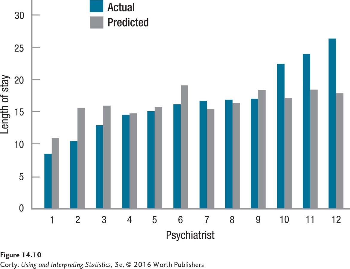
How could one tell if a psychiatrist were assigned difficult or easy patients? Difficult patients should have a longer predicted length of stay. So, calculating the mean predicted length of stay for each psychiatrist should answer that question. The grey bars in Figure 14.10 show the mean predicted length of stay corresponding to each psychiatrist.
Look at Psychiatrist 1. Earlier, when the focus was only on the blue bars showing actual length of stay, he appeared to be doing a good job because his patients had the shortest length of stay. Now, looking at the grey bar, it is apparent that this psychiatrist was assigned the healthiest patients. No wonder he discharged them quickly.
560
The two bars, one the actual length of stay and the other predicted by multiple regression, allow us to think about this psychiatrist’s performance in a more complex fashion. Psychiatrist 1’s patients have a mean length of stay around 8 days but are predicted to need approximately 11 days. Why the difference? There are three likely explanations, two of which involve his skills and one that involves multiple regression. First, perhaps he is a phenomenal psychiatrist and cures people quickly. It could happen. Second, maybe he is a terrible psychiatrist who can’t assess patients’ progress and discharges them before they are ready. That could happen, too. Third, maybe there are errors in prediction. Maybe this is especially true for the healthier cases and their lengths of stay are overestimated.
Whatever the explanation turns out to be, this study shows how multiple regression is used in psychology and how predictions are made and utilized. Regression, either simple or multiple, is a useful tool that helps researchers understand their results in more detail.