CHAPTER EXERCISES
562
Answers to the odd-numbered exercises appear in Appendix B.
Review Your Knowledge
14.01 The correlation chapter was about understanding ____ between variables; this chapter, on regression, is about ____ one ____ from another ____.
14.02 In linear regression, the ____ variable is X and Y is the ____ variable.
14.03 It is reasonable to do linear regression if the correlation between X and Y is ____.
14.04 ____ is the abbreviation for a predicted value of Y.
14.05 If blindly guessing a person’s score, the best guess is the ____.
14.06 Statisticians use the ____ criterion to judge the regression line.
14.07 On the basis of least squares, the best-fitting line is the one that ____ the sum of the ____.
14.08 The difference between a case’s actual Y score and its predicted Y score is called a ____.
14.09 A residual score is a measure of ____.
14.10 In the linear regression equation, b is the ____ and a is the ____.
14.11 Y′ in the regression equation is ____ and X is the ____.
14.12 A ____ slope means the line is moving down and to the right.
14.13 If the correlation is positive, the slope of the regression line is ____.
14.14 If a slope is –0.50, then for every 1-point increase in X, there is a 0.5-point ____ in Y.
14.15 The spot where the regression line would pass through the ____ is called the Y-intercept.
14.16 Predictions of Y from X should only be made for X values that fall within the range of ____ used to develop the regression equation.
14.17 If X = 17 and Y′ = 29.37, then the value 29.37 is a ____ estimate.
14.18 An ____ estimate is better than a ____ estimate.
14.19 If one uses a regression equation to predict Y′ from X, and several cases have the same X value, then each time Y′ is predicted for these cases, Y′ will be the same / different.
14.20 The standard deviation of the residual scores is called the ____.
14.21 The standard error of the estimate can be thought of as the average ____ in prediction.
14.22 A prediction interval gives the range within which it is likely that a case’s Y / Y′ value falls.
14.23 The standard error of the estimate has an impact on the ____ of a prediction interval.
14.24 Simple regression uses ____ predictor variable to predict Y′; multiple regression uses ____.
14.25 Comparing multiple regression to simple regression, ____ usually accounts for a higher percentage of variability in Y than does ____.
14.26 Multiple regression is often used in college ____ decisions.
Apply Your Knowledge
Using regression lines to predict Y
14.27 Given this regression line, predict Y for an X value of 30:
563
14.28 Given this regression line, predict Y for X = 25:
Calculating slope
14.29 If r = –.47, sY = 3.65, and sX = 9.66, what is b?
14.30 If r = .28, sY = 0.34, and sX = 0.28, what is b?
Interpreting slope
14.31 An automotive magazine used the price of gas in cents per gallon to predict the number of miles families drove on their summer vacations. The slope of the regression line was –35. Use the slope to interpret the impact of gas prices on vacation driving.
14.32 An exercise physiologist used the number of hours of TV watched per week at age 30 to predict the number of pounds gained over the next 10 years. The slope of the regression line was 1.25. Use the slope to interpret the impact of watching TV on weight gain.
Calculating the Y-intercept
14.33 If b = 4.33, MX = 5.00, and MY = 17.50, what is a?
14.34 If b = –2.45, MX = 53.45, and MY = 112.23, what is a?
Forming a regression equation
14.35 Given b = 12.98 and a = –5.00, write a regression equation.
14.36 Given b = –0.68 and a = 7.50, write a regression equation.
14.37 Given r = –.24, MX = 55.00, sX = 11.00, MY = 25.00, and sY = 3.98, write a regression equation.
14.38 Given r = .33, MX = 2.50, sX = 1.50, MY = 112.50, and sY = 21.50, write a regression equation.
Predicting Y
14.39 Find Y′ if X = 25 for Y′ = 0.37X + 15.
14.40 Find Y′ if X = –10 for Y′ = 13X + 88.
Drawing a regression line
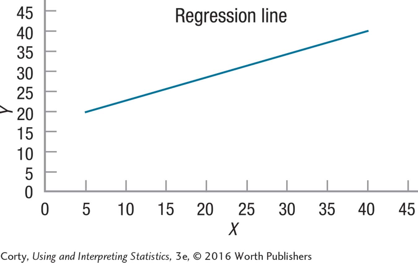
14.41 (a) Given the endpoints of (10, 20) and (80, 50), draw a regression line. (b) What is the range of X values for which Y′ can be calculated?
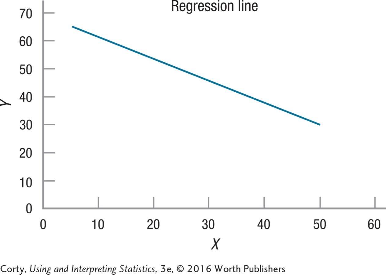
14.42 (a) Given the endpoints of (0, 70) and (50, 0), draw a regression line. (b) What is the range of X values for which Y′ can be calculated?
14.43 Here is a regression equation: Y′ = 2.50 X – 12.50. If X values can range from 30 to 70, draw the regression line.
14.44 Here is a regression equation: Y′ = –1.10X + 115. If X values can range from 70 to 130, draw the regression line.
Calculating residual scores
14.45 If X = 75.45, Y = 12.96, and Y′ = 13.43, what is the residual score?
14.46 If X = 24.77, Y = 33.43, and Y′ = 31.22, what is the residual score?
Calculating standard error of the estimate
14.47 If r = .28 and sY = 10.55, what is the standard error of the estimate?
14.48 If r = .20 and sY = 30.42, what is the standard error of the estimate?
Interpreting standard error of the estimate
14.49 Dr. Lansing is using high school GPA to predict combined SAT scores. Combined SAT scores from the two SAT subtests can range from 400 to 1600. He calculated the standard error of the estimate as 40. Interpret this error of the estimate.
14.50 Dr. Pallas is predicting severity of depression in adulthood from a childhood behavior checklist. The severity of depression scale ranges from 0 to 50 and the standard error of the estimate is 2.25. Interpret this error of the estimate.
564
Calculating Y′ in multiple regression
14.51 A multiple regression equation has a constant of 5.74, a weight of 3.42 for variable 1, and a weight of –0.76 for variable 2. If a case has a score of 56.66 on variable 1 and a score of 88.99 on variable 2, what is Y′?
14.52 A multiple regression equation has a constant of 25.12, a weight of –4.55 for variable 1, a weight of –8.86 for variable 2, and a weight of 10.76 for variable 3. If a case has a score of 7.33 on variable 1, a score of 12.20 on variable 2, and a score of 18.85 on variable 3, what is Y′?
Expand Your Knowledge
14.53 Jeff is an above-average golfer. He decides to change sports and take up ping pong. If there is a strong, positive correlation between golf ability and ping pong ability, predict how he’ll perform as a ping pong player?
Excellent
Above average
Average
Below average
Terrible
Not enough information given to reach a conclusion.
Ping pong and golf are different sports and one can’t be predicted from the other.
14.54 Sue is an above-average golfer. She decides to change sports and take up archery. If a strong, negative correlation exists between golf ability and archery ability, predict how she’ll perform as an archer?
Excellent
Above average
Average
Below average
Terrible
Not enough information given to reach a conclusion.
Archery and golf are different sports and one can’t be predicted from the other.
14.55 David is an above-average golfer. He decides to change sports and take up wrestling. If there is a no correlation between golf ability and wrestling ability, predict how he’ll rate as a wrestler?
Excellent
Above average
Average
Below average
Terrible
Not enough information given to reach a conclusion.
14.56 Shemekia applied to a college that uses multiple regression to select students. This college only considers students whose predicted first-year GPA is 3.0 or higher. Shemekia’s predicted GPA was 2.9, and she did not get accepted. The correlation between the predictor variable and GPA is .30 and the standard deviation for GPA is .40. Based on this, what argument could Shemekia make to the college for why she should be considered?
14.57 Continue with Exercise 14.56. The college responds to Shemekia. Based on the same information, what argument could the college make for why she shouldn’t be offered admission?
14.58 If Y′ and sY–Y′ are known, make an educated guess as to what the 95% prediction interval would be.
14.59 There is a graph with a regression line for predicting Y. Could it be used to predict X?
565
SPSS
SPSS does calculate linear regression. We’ll use Dr. Paik’s marital satisfaction data to show how it works. Figure 14.11 illustrates how the data are arranged with each variable (role flexibility and marital satisfaction) in its own column and each case in its own row.
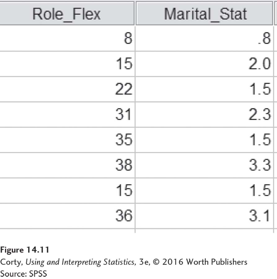
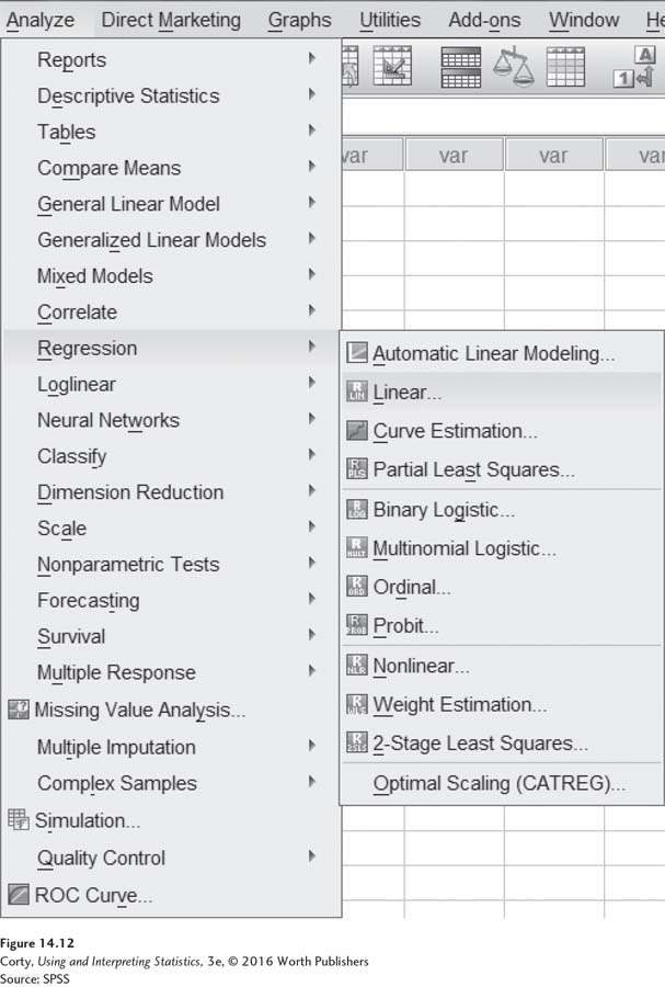
Figure 14.12 shows how to access the linear regression commands in SPSS. Click on “Analyze,” then “Regression,” and finally “Linear.” SPSS calls the predictor variable “independent” and the outcome variable “dependent.”
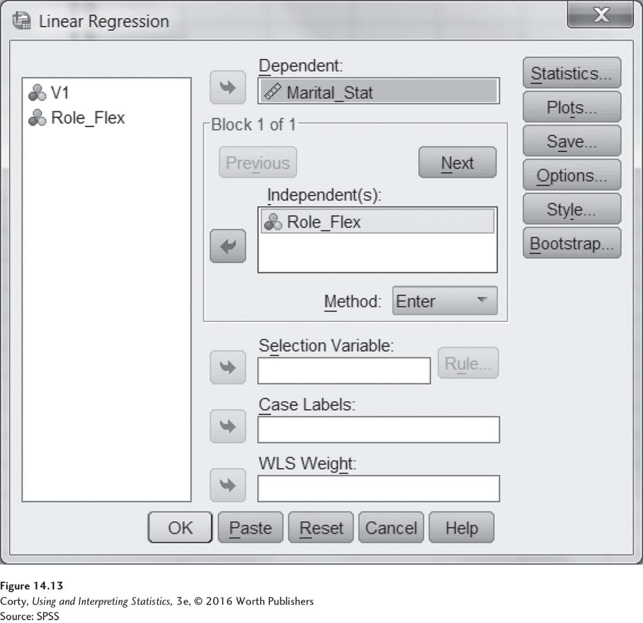
Clicking on “Linear” opens up the commands seen in Figure 14.13. Notice that Y, the dependent variable “Marital_Sat,” has been moved over to be the dependent variable. Also, X, the independent variable “Role_Flex,” has been moved over to be an independent variable. Clicking on “OK” in the lower right starts the calculations.
566
The output, of which SPSS generates a lot, is shown in Figure 14.14. First, look in the table named “Model Summary.” There, it says “R = .762.” R is the value of the correlation coefficient. (R is the abbreviation for a multiple regression. We’ve borrowed it to do a simple regression and SPSS can’t tell.)
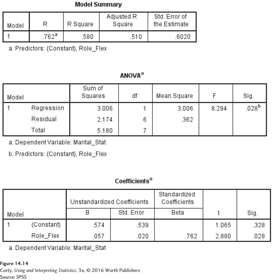
SPSS carries many more decimal places than this text does, so its answers will differ from the answers here. The slope of the line, which was calculated as 0.06 in the text, is 0.057 in SPSS and is found next to the predictor variable, “Role_Flex” under the “B” column under “Unstandardized coefficients.” The Y-intercept, which was calculated as 0.50 in the text, is 0.574 in SPSS and is found in the same column in the row labeled “(Constant).”