7.2 Interpreting the Single-Sample t Test
 StatClips: Confidence Interval Intro Part IVideo on LaunchPad
StatClips: Confidence Interval Intro Part IIVideo on LaunchPad
StatClips: Confidence Intervals: InterpretationVideo on LaunchPad
StatClips: Confidence Interval Intro Part IIIVideo on LaunchPad
StatClips: Using Confidence Intervals to Make DecisionsVideo on LaunchPad
Computers are great for statistics. They can crunch numbers and do math faster and more accurately than humans can. But even a NASA supercomputer couldn’t do what we are about to do: use common sense to explain the results of a single-sample t test in plain English. Interpretation is the most human part of statistics.
Interpretation is the most human part of statistics.
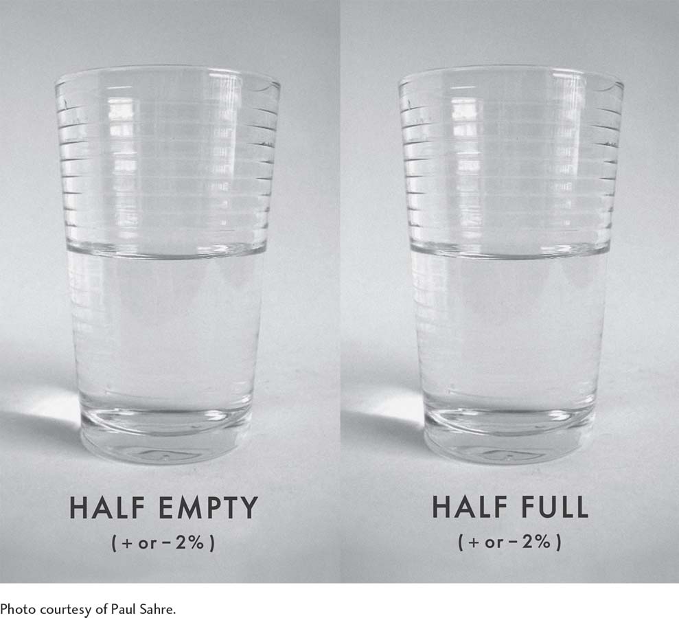
To some degree, interpretation is a subjective process. The researcher takes objective facts—like the means and the test statistic—and explains them in his or her own words. How one researcher interprets the results of a hypothesis test might differ from how another researcher interprets them. Reasonable people can disagree. But, there are guidelines that researchers need to follow. An interpretation needs to be supported by facts. One person may perceive a glass of water as half full and another as half empty, but they should agree that it contains roughly equal volumes of water and air.
229
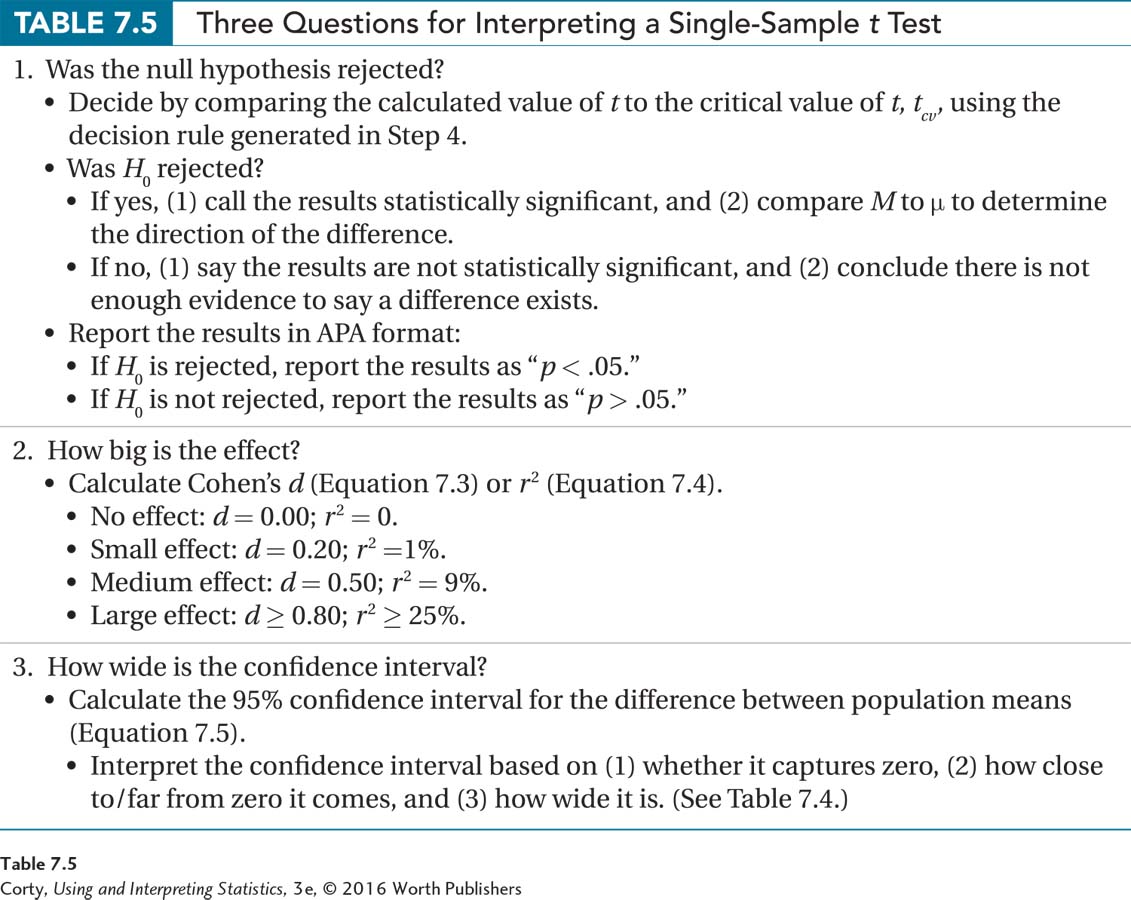
Interpreting the results of a hypothesis test starts with questions to be answered. The answers will provide the material to be used in a written interpretation. For a single-sample t test, our three questions are:
Was the null hypothesis rejected?
How big is the effect?
How wide is the confidence interval?
The questions are sequential. Each one gives new information that is useful in understanding the results from a different perspective. Answering only the first question, as was done in the last chapter, will provide enough information for completing a basic interpretation. However, answering all three questions leads to a more nuanced understanding of the results and a better interpretation.
Let’s follow Dr. Farshad as she interprets the results of her study, question by question. But, first, let’s review what she did. Dr. Farshad wondered if adults with ADHD differed in reaction time from the general population. To test this, she obtained a random sample, from her state, of 141 adults who had been diagnosed with ADHD. She had each participant take a reaction time test and found the sample mean and sample standard deviation (M = 220 msec, s = 27 msec). She planned to use a single-sample t test to compare the sample mean to the population mean for adult Americans (μ = 200 msec).
Dr. Farshad’s hypotheses for the single-sample t test were nondirectional as she was testing whether adults with ADHD had faster or slower reaction times than the general population. She was willing to make a Type I error no more than 5% of the time, she was doing a two-tailed test, and she had 140 degrees of freedom, so the critical value of t was ±1.977. The first step in calculating t was to find the estimated standard error of the mean (sM = 2.21) and she used that in order to go on and find t = 8.81.
Step 6 Interpret the Results
Was the Null Hypothesis Rejected?
In Dr. Farshad’s study, the t value was calculated as 8.81. Now it is time to decide whether the null hypothesis was rejected or not. To do so, Dr. Farshad puts the t value, 8.81, into the decision rule that was generated for the critical value of t, ±1.977, in Step 4. Which of the following statements is true?
Is 8.81 ≤ –1.977 or is 8.81 ≥ 1.977?
Is –1.977 < 8.81 < 1.977?
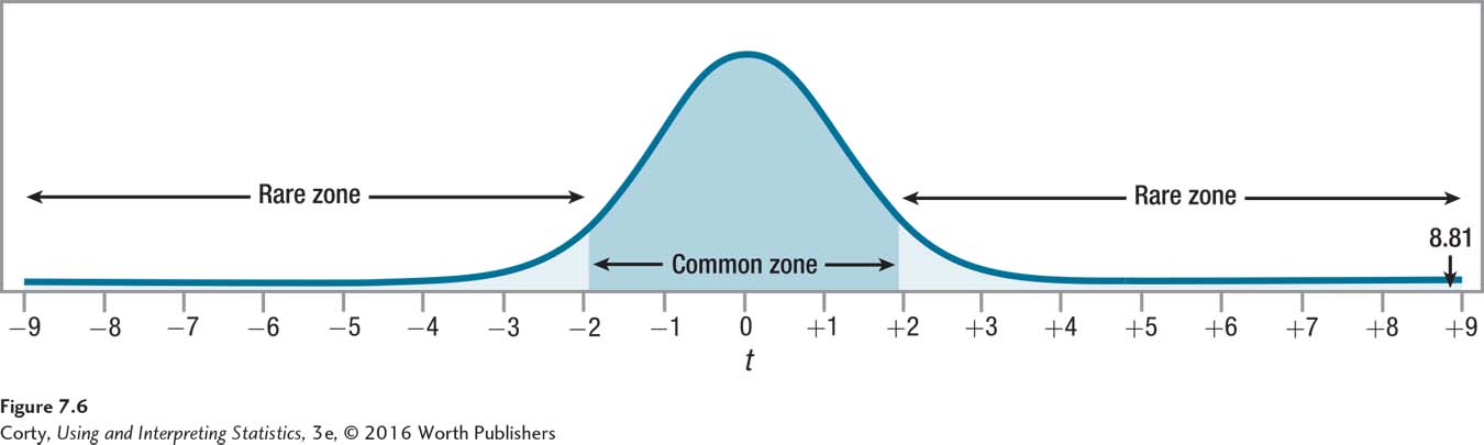
The second part of the first statement is true: 8.81 is greater than or equal to 1.977. The observed value of t, 8.81, falls in the rare zone of the sampling distribution, so the null hypothesis is rejected (see Figure 7.6). She can conclude that there is a statistically significant difference between the sample mean of the adults with ADHD and the general population mean.
Rejecting the null hypothesis means that Dr. Farshad has to accept the alternative hypothesis and conclude that the mean reaction time for adults with ADHD is different from the mean reaction time for the general population. Now she needs to determine the direction of the difference. By comparing the sample mean (220) to the population mean (200), she can conclude that adults with ADHD take a longer time to react and so have a slower reaction time than adults in general.
Dr. Farshad should also report the results in APA format. APA format provides five pieces of information: (1) what test was done, (2) the number of cases, (3) the value of the test statistic, (4) the alpha level used, and (5) whether the null hypothesis was or wasn’t rejected.
230
In APA format, the results would be t(140) = 8.81, p < .05:
The initial t says that the statistical test was a t test.
The sample size, 141, is present in disguised form. The number 140, in parentheses, is the degrees of freedom for the t test. For a single-sample t test, df = N – 1. That means N = df + 1. So, if df = 140, N = 140 + 1 = 141.
The observed t value, 8.81, is reported. This number is the value of t calculated, not the critical value of t found in Appendix Table 3. Note that APA format requires the value to be reported to two decimal places, no more and no fewer.
The .05 tells that alpha was set at .05.
The final part, p < .05, reveals that the null hypothesis was rejected. It means that the observed result (8.81) is a rare result—it has a probability of less than .05 of occurring when the null hypothesis is true.
If Dr. Farshad stopped after answering only the first interpretation question, this is what she could write for an interpretation:
There is a statistically significant difference between the mean reaction time of adults in Illinois with ADHD and the reaction time found in the general U.S. population, t(140) = 8.81, p < .05. Adults with ADHD (M = 220 msec) have a slower mean reaction time than does the general public (μ = 200).
Practice Problems 7.2
Apply Your Knowledge
For these problems, use α = .05, two-tailed.
7.10 If N = 19 and t = 2.231, write the results in APA format.
7.11 If N = 7 and t = 2.309, write the results in APA format.
7.12 If N = 36 and t = 2.030, write the results in APA format.
7.13 If N = 340 and t = 3.678, write the results in APA format.
How Big Is the Effect?
231
All we know so far is that there is a statistically significant difference, such that we can conclude that adults with ADHD in Illinois have slower reaction times than the general American adult population does. We know there’s a 20-msec difference, but we are hard-pressed to know how much of a difference that really is.
Thus, the next question to address when interpreting the results is effect size, how large the impact of the explanatory variable is on the outcome variable. With the reaction-time study, the explanatory variable is ADHD status (adults with ADHD vs. the general population) and the outcome variable is reaction time. Asking what the effect size is, is asking how much impact ADHD has on a person’s reaction time.
In this section, we cover two ways to measure effect size: Cohen’s d and r2. Both can be used to determine if the effect is small, medium, or large. Both standardize the effect size, so outcome variables measured on different metrics can be compared. A 2-point change in GPA would be huge, while a 2-point change in total SAT score would be trivial. Both Cohen’s d and r2 take the unit of measurement into account. And, finally, both will be used as measures of effect size for other statistical tests in other chapters.
Cohen’s d
The formula for Cohen’s d is shown in Equation 7.3. It takes the difference between the two means and standardizes it by dividing it by the sample standard deviation. Thus, d is like a z score—it is a standard score that allows different effects measured by different variables in different studies to be expressed—and compared—with a common unit of measurement.
Equation 7.3 Formula for Cohen’s d for a Single-Sample t Test
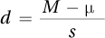
where d = the effect size
M = sample mean
μ = hypothesized population mean
s = sample standard deviation
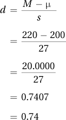
To calculate d, Dr. Farshad needs to know the sample mean, the population mean, and the sample standard deviation. For the reaction-time data, M = 220, μ = 200, and s = 27. Here are her calculations for d:
232
Cohen’s d = 0.74 for the ADHD reaction-time study. Follow APA format and use two decimal places when reporting d. And, because d values can be greater than 1, values of d from –0.99 to 0.99 get zeros before the decimal point.
In terms of the size of the effect, it doesn’t matter whether d is positive or negative. A d value of 0.74 indicates that the two means are 0.74 standardized units apart. This is an equally strong effect whether it is 0.74 or –0.74. But the sign associated with d is important for knowing the direction of the difference, so make sure to keep it straight.
Here’s how Cohen’s d works:
A value of 0 for Cohen’s d means that the explanatory variable has absolutely no effect on the outcome variable.
As Cohen’s d gets farther away from zero, the size of the effect increases.
Cohen (1988), the developer of d, has offered standards for what small, medium, and large effect sizes are in the social and behavioral sciences. Cohen’s d values for these are shown in Table 7.3. In Figure 7.7, the different effect sizes are illustrated by comparing the IQ of a control group (M = 100) to the IQ of an experimental group that is smarter by the amount of a small effect (3 IQ points), a medium effect (7.5 IQ points), or a large effect (12 IQ points).
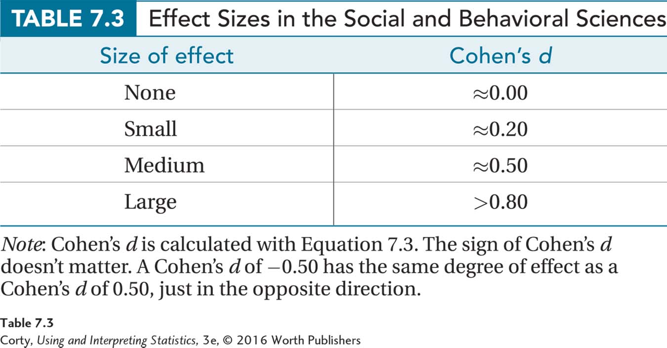
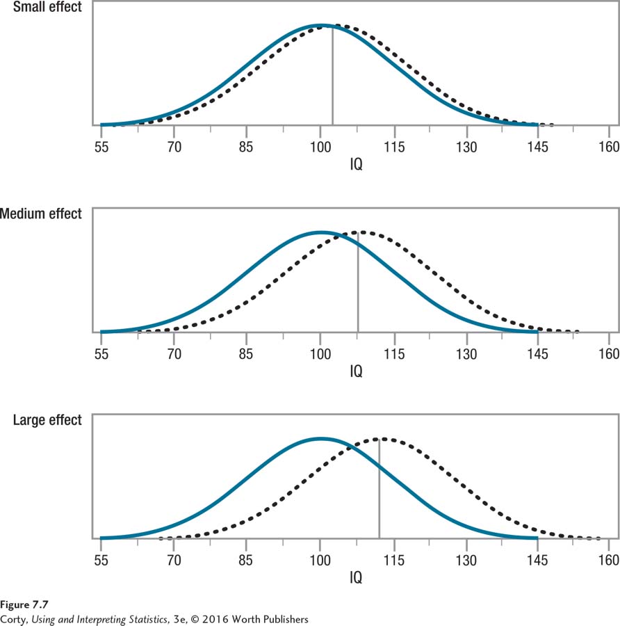
Cohen describes a small effect as a d of around 0.20. This occurs when there is a small difference between means, a difference in performance that would not be readily apparent in casual observation. Look at the top panel in Figure 7.7. That’s what a small effect size looks like. Though the two groups differ by 3 points on intelligence (M = 100 vs. M = 103), it wouldn’t be obvious that one group is smarter than the other without using a sensitive measure like an IQ test (Cohen, 1988).
Another way to visualize the size of the effect is to consider how much overlap exists between the two groups. If the curve for one group fits exactly over the curve for the other, then the two groups are exactly the same and there is no effect. As the amount of overlap decreases, the effect size increases. For the small effect in Figure 7.7, about 85% of the total area overlaps.
A medium effect size, a Cohen’s d of around 0.50, is large enough to be observable, according to Cohen. Look at the middle panel in Figure 7.7. One group has a mean IQ of 100, and the other group has a mean IQ of 107.5, a 7.5 IQ point difference. Notice the amount of differentiation between groups for a medium effect size. In this example, about two-thirds of the total area overlaps, a decrease from the 85% overlap seen with a small effect size.
233
A large effect size is a Cohen’s d of 0.80 or larger. This is shown in the bottom panel of Figure 7.7. One group has a mean IQ of 100, and the other group has a mean IQ of 112, a 12 IQ point difference. Here, there is a lot of differentiation between the two groups with only about half of the area overlapping. The increased differentiation can be seen in the large section of the control group that has IQs lower than the experimental group and the large section of the experimental group that has IQs higher than the control group.
The Cohen’s d calculated for the reaction-time study by Dr. Farshad was 0.74, which means it is a medium to large effect. If she stopped her interpretation after calculating this effect size, she could add the following sentence to her interpretation: “The effect of ADHD status on reaction time falls in the medium to large range, suggesting that the slower mean reaction time associated with having ADHD may impair performance.”
234
r Squared
The other commonly used measure of effect size is r2. Its formal name is coefficient of determination, but everyone calls it r squared. r2, like d, tells how much impact the explanatory variable has on the outcome variable.
Equation 7.4 Formula for r2, the Percentage of Variability in the Outcome Variable Accounted for by the Explanatory Variable
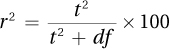
where r2 = the percentage of variability in the outcome variable that is accounted for by the explanatory variable
t2 = the squared value of t from Equation 7.2
df = the degrees of freedom for the t value
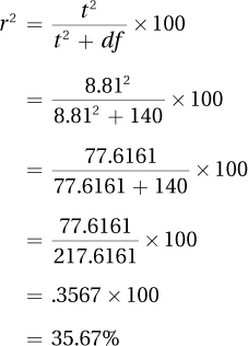
This formula says that r2 is calculated as the squared t value divided by the sum of the squared t value plus the degrees of freedom for the t value. Then, to turn it into a percentage, the ratio is multiplied by 100. r2 can range from 0% to 100%. These calculations reveal the percentage of variability in the outcome scores that is accounted for (or predicted) by the explanatory variable. For the ADHD data, these calculations would lead to the conclusion that r2 = 36%:
r2 tells the percentage of variability in the outcome variable that is accounted for (or predicted) by the explanatory variable.
What does r2 tell us? Imagine that someone took a large sample of people and timed them running a mile. There would be a lot of variability in time, with some runners taking 5 minutes and others 20 minutes or more. What are some factors that influence running speed? Certainly, physical fitness and age play important roles, as do physical health and weight. Which of these four factors has the most influence on running speed? That could be determined by calculating r2 for each variable. The factor that has the largest r2, the one that explains the largest percentage of variability in time, has the most influence.
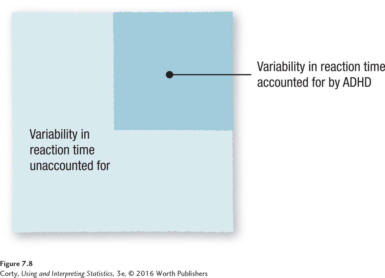
The question addressed by r2 in the reaction-time study is how much of the variability in reaction time is accounted for by the explanatory variable (ADHD status) and how much is left unaccounted for:
The closer r2 is to 100%, the stronger the effect of the explanatory variable is and the less variability in the outcome variable remains to be explained by other variables.
235
The closer r2 is to 0%, the weaker the effect of the explanatory variable and the more variability in the dependent variable exists to be explained by other variables.
Cohen (1988), who provided standards for d values, also provides standards for r2:
A small effect is an r2 ≈ 1%.
A medium effect is an r2 ≈ 9%.
A large effect is an r2 ≈ 25%.
By Cohen’s standards, an r2 of 36%, as is the case in our ADHD study, is a large effect. This means that as far as explanatory variables in the social and behavioral sciences go, this one accounts for a lot of the variability in the outcome variable. Figure 7.8 is a visual demonstration of what explaining 36% of the variability means. Note that although a majority of the variability, 64%, in reaction time remains unaccounted for, this is still considered a large effect. Here is what Dr. Farshad could add to her interpretation now that r2 is known: “Having ADHD has a large effect on one’s reaction time. In the present study, knowing ADHD status explains more than a third of the variability in reaction time.”
One important thing to note is that even though Dr. Farshad went to the trouble of calculating both d and r2, it is not appropriate to report both. These two provide overlapping information and it does not make a case stronger to say that the effect was a really strong one, because both d and r2 are large. This would be like testing boiling water and reporting that it was really, really boiling because it registered 212 degrees on a Fahrenheit thermometer and 100 degrees on a Celsius thermometer.
Here’s a heads up for future chapters and for reading results sections in psychology articles—there are other measures of effect size that are similar to r2. Both η2 (eta squared) and ω2 (omega squared) provide the same information, how much of the variability in the outcome variable is explained by the explanatory variable.
236
Practice Problems 7.3
Apply Your Knowledge
7.14 If M = 66, μ = 50, and s = 10, what is d?
7.15 If M = 93, μ = 100, and s = 30, what is d?
7.16 If N = 18 and t = 2.37, what is r2?
7.17 If r = .32, how much of the variability in the outcome variable, Y, is accounted for by the explanatory variable, X?
How Wide Is the Confidence Interval?
In Chapter 5, we encountered confidence intervals for the first time. There, they were used to take a sample mean, M, and estimate a range of values that was likely to capture the population mean, μ. Now, for the single-sample t test, the confidence interval will be used to calculate the range for how big the difference is between two population means. Two populations? Dr. Farshad’s confidence interval, in the ADHD reaction-time study, will tell how large (or small) the mean difference in reaction time might be between the population of adults with ADHD and the general population of Americans.
The difference between population means can be thought of as an effect size. If the distance between two population means is small, then the size of the effect (i.e., the impact of ADHD on reaction time) is not great. If the two population means are far apart, then the size of the effect is large.
Equation 7.5 is the formula for calculating a confidence interval for the difference between two population means. It calculates the most commonly used confidence interval, the 95% confidence interval.
Equation 7.5 95% Confidence Interval for the Difference Between Population Means
95% CIμDiff = (M – μ) ± (tcv × sM)
where 95% CIμDiff = the 95% confidence interval for the difference between two population means
M = sample mean from one population
μ = mean for other population
tcv = critical value of t, two-tailed, α = .05, df = N – 1 (Appendix Table 3)
sM = estimated standard error of the mean (Equation 5.2)
Here are all the numbers Dr. Farshad needs to calculate the 95% confidence interval:
M, the mean for the sample of adults with ADHD, is 220.
μ, the population mean for adults in general, is 200.
sM = 2.27, a value obtained earlier via Equation 5.2 for use in Equation 7.2.
tcv, the critical value of t, is 1.977.
237
Applying Equation 7.5, she would calculate
95% CIμDiff = (M – μ) ± (tcv × sM)
= (220 – 200) ± (1.977 × 2.27)
= 20.0000 ± 4.4878
= from 15.5122 to 24.4878
= from 15.51 to 24.49
The 95% confidence interval for the difference between population means ranges from 15.51 msec to 24.49 msec. In APA format, this confidence interval would be reported as 95% CI [15.51, 24.49].
What information does a confidence interval provide? The technical definition is that if one drew sample after sample and calculated a 95% confidence interval for each one, 95% of the confidence intervals would capture the population value. But, that’s not very useful as an interpretative statement. Two confidence interval experts have offered their thoughts on interpreting confidence intervals (Cumming and Finch, 2005). With a 95% confidence interval, one interpretation is that a researcher can be 95% confident that the population value falls within the interval. Another way of saying this is that the confidence interval gives a range of plausible values for the population value. That means it is possible, but unlikely, that the population value falls outside of the confidence interval. A final implication is that the ends of the confidence interval are reasonable estimates of how large or how small the population value is. The end of the confidence interval closer to zero can be taken as an estimate of how small the population value might be, while the end of the confidence interval further from zero estimates how large the population value might be.
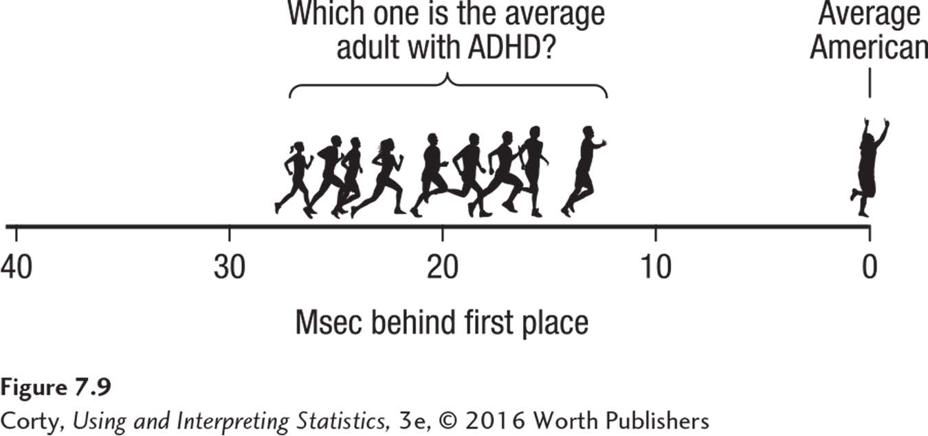
Dr. Farshad’s confidence interval tells her that there’s a 95% chance that the difference between the two population means falls somewhere in the interval from 15.51 msec to 24.49 msec. It means that the best prediction of how much slower reaction times are for the population of adults with ADHD than for the general population of Americans ranges from 15.51 msec slower to 24.49 msec slower (Figure 7.9).
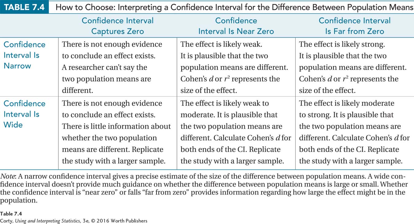
Our interpretation of confidence intervals will focus on three aspects: (1) whether the value of 0 falls within the confidence interval; (2) how close the confidence interval comes to zero or how far from zero it goes, and (3) how wide the confidence interval is. These three aspects are explained below and summarized in Table 7.4.
238
Does the confidence interval capture zero? The 95% confidence interval for the difference between population means gives the range within which it is likely that the actual difference between two population means lies. If the null hypothesis is rejected for a single-sample t test, the conclusion reached is that this sample probably did not come from that population; rather, that there are two populations with two different means. In such a situation, the difference between the two population means is not thought to be zero, and the confidence interval shouldn’t include zero. When the null hypothesis is rejected, the 95% confidence interval won’t capture zero. (This assumes that the researcher was using a two-tailed test with α = .05.)
However, when a researcher fails to reject the null hypothesis, the confidence interval should include zero in its range. All that a zero falling in the range of the confidence interval means is that it is possible the difference between the two population means is zero. It doesn’t mean that the difference is zero, just that it may be. In a similar fashion, when one fails to reject the null hypothesis, the conclusion is that there isn’t enough evidence to say the null hypothesis is wrong. It may be right, it may be wrong; the researcher just can’t say.
Having already determined earlier that the null hypothesis was rejected and the results were statistically significant, Dr. Farshad knew that her confidence interval wouldn’t capture zero. And, as the interval ranged from 15.51 to 24.49, she was right.
How close does the confidence interval come to zero? How far away from zero does it go? If the confidence interval doesn’t capture zero, how close one end of the confidence interval comes to zero can be thought of as providing information about how weak the effect may be. If one end of the confidence interval is very close to zero, then the effect size may be small, as there could be little difference between the population means.
Similarly, how far away the other end of the confidence interval is from zero can be thought of as providing information about how strong the effect may be. The farther away from zero the confidence interval ranges, the larger the effect size may be.
239
How wide is the confidence interval? The width of the confidence interval also provides information. Narrower confidence intervals provide a more precise estimate of the population value and are more useful.
When the confidence interval is wide, the size of the effect in the population is uncertain. It might be a small effect, a large effect, or anywhere in between. In these instances, replication of the study with a larger sample size will yield a narrower confidence interval.
When evaluating the width of a confidence interval, one should take into account the variable being measured. A confidence interval that is 1 point wide would be wide if the variable were GPA, but narrow if the variable were SAT. Interpretation relies on our human common sense.
Dr. Farshad’s confidence interval ranges from 15.51 to 24.49. The width can be determined by subtracting the lower limit from the upper limit, as shown in Equation 7.6.
Equation 7.6 Formula for Calculating the Width of a Confidence Interval
CIW = CIUL – CILL
where CIW = the width of the confidence interval
CIUL = the upper limit of the confidence interval
CILL = the lower limit of the confidence interval
Applying Equation 7.6 to her data, Dr. Farshad calculates 24.49 – 15.51 = 8.98. The confidence interval is almost 9 msec wide. Is this wide or narrow?
Evaluating the width of a confidence interval often requires expertise. It takes a reaction-time researcher like Dr. Farshad to tell us whether a 9-msec range for a confidence interval is a narrow range and sufficiently precise. Here, given the width of the confidence interval, she feels little need to replicate the study with a larger sample size to narrow the confidence interval.
Putting It All Together
Dr. Farshad has completed her study using a single-sample t test to see if adults with ADHD had a reaction time that differed from that for the general population. By addressing the three questions in Table 7.5, Dr. Farshad has gathered all the pieces she needs to write an interpretation. There are four points she addresses in her interpretation:
Dr. Farshad starts with a brief explanation of the study.
She presents some facts, such as the means of the sample and the population. But, she does not report all the values she calculated just because she calculated them. Rather, she is selective and only reports what she believes is most relevant.
She explains what she believes the results mean.
Finally, she offers some suggestions for future research. Having been involved in the study from start to finish, she knows its strengths and weaknesses better than anyone else. She is in a perfect position to offer advice to other researchers about ways to redress the limitations of her study. In her suggestions, she uses the word “replicate.” To replicate a study is to repeat it, usually introducing some change in procedure to make it better.
240
Here is Dr. Farshad’s interpretation:
A study compared the reaction time of a random sample of Illinois adults who had been diagnosed with ADHD (M = 220 msec) to the known reaction time for the American population (μ = 200 msec). The reaction time of adults with ADHD was statistically significantly slower than the reaction time found in the general population [t(140) = 8.81, p < .05]. The size of the difference in the larger population probably ranges on this task from a 16- to a 24-msec decrement in performance. This is not a small difference—these results suggest that ADHD in adults is associated with a medium to large level of impairment on tasks that require fast reactions. If one were to replicate this study, it would be advisable to obtain a broader sample of adults with ADHD, not just limiting it to one state. This would increase the generalizability of the results.
Worked Example 7.2
For practice in interpreting the results of a single-sample t test when the null hypothesis is not rejected, let’s return to Dr. Richman’s study.
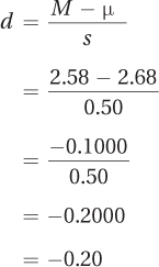
In his study, Dr. Richman studied the effect of losing a pet during the year on college performance. Dr. Richman located 11 students who had lost a pet. Their mean GPA for the year was 2.58 (s = 0.50) compared to a population mean of 2.68. Because he expected pet loss to have a negative effect, Dr. Richman used a one-tailed test. With the alpha set at .05, tcv was –1.812. He calculated sM = 0.15 and found t = –0.67. Now it is time for Dr. Richman to interpret the results.
241
Was the null hypothesis rejected? The vet was doing a one-tailed test and his hypotheses were
H0: μStudentsWithPetLoss ≥ 2.68
H1: μStudentsWithPetLoss < 2.68
Inserting the observed value of t, –0.67, into the decision rule he had generated in Step 4, he has to decide which statement is true:
Is –0.67 ≤ –1.812? If so, reject H0.
Is –0.67 > –1.812? If so, fail to reject H0.
As the second statement is true, Dr. Richman has failed to reject the null hypothesis. Figure 7.10 shows how the t value of –0.67 falls in the common zone of the sampling distribution.
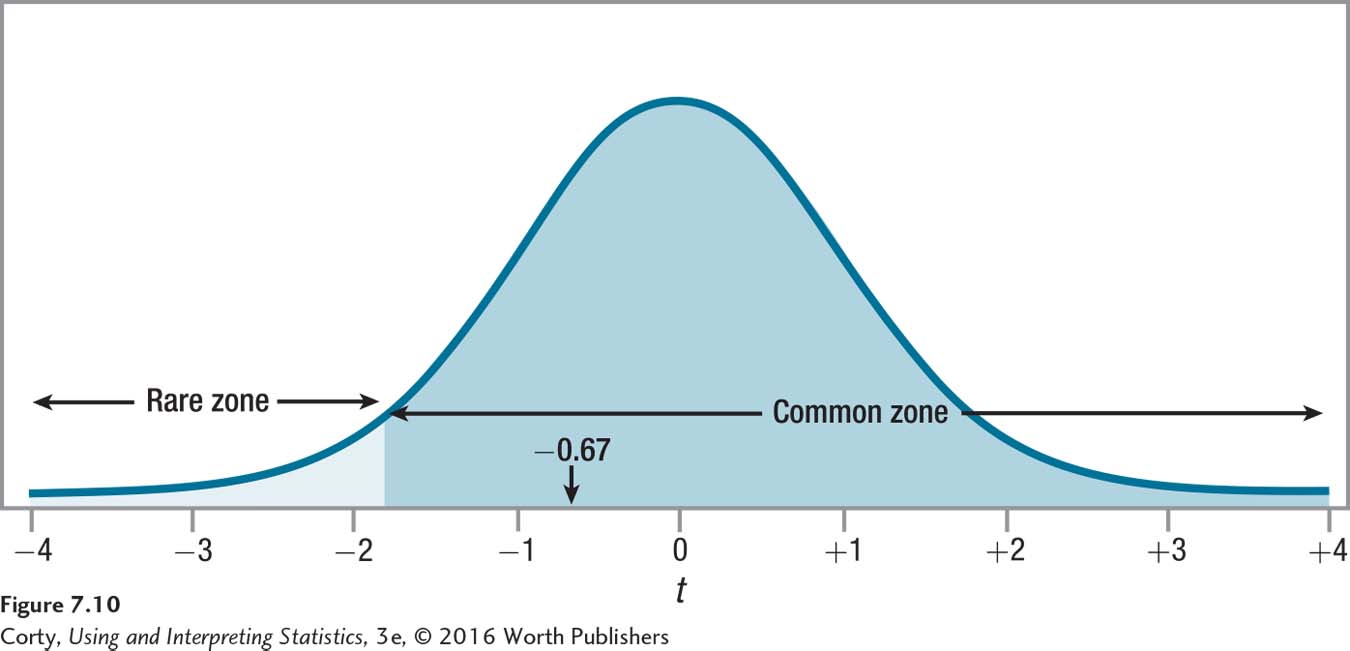
Having failed to reject the null hypothesis, the results are called not statistically significant. Just like finding a defendant not guilty doesn’t mean that the defendant is innocent, failing to reject the null hypothesis does not mean that it is true. All the vet can conclude is that there’s not enough evidence to conclude that college students who lose a pet do worse in school that year. Because he failed to reject the null hypothesis, there’s no reason to believe a difference exists between the two populations, and there’s no reason for him to worry about the direction of the difference between them.
In APA format, the results would be written as t(10) = –0.67, p > .05 (one-tailed):
The t tells what statistical test was done.
The 10 in parentheses, which is the degrees of freedom, reveals there were 11 cases as N = df + 1 for a single-sample t test.
–0.67 is the observed value of the statistic.
The .05 indicates that this was the alpha level selected.
p > .05 indicates that the researcher failed to reject the null hypothesis. The observed t value is a common one when the null hypothesis is true. “Common” is defined as occurring more than 5% of the time.
242
The final parenthetical expression (one-tailed) is something new. It indicates, obviously, that the test was a one-tailed test. Unless told that the test is a one-tailed test, assume it is two-tailed.
How big is the effect? Calculating an effect size like Cohen’s d or r2 when one has failed to reject the null hypothesis is a controversial topic in statistics. If one fails to reject the null hypothesis, not enough evidence exists to state there’s an effect. Some researchers say that there is no need to calculate an effect size if no evidence that an effect exists is found. Other researchers believe that examining the effect size when one has failed to reject the null hypothesis alerts the researcher to the possibility of a Type II error (Cohen, 1994; Wilkinson, 1999). (Remember, a Type II error occurs when the null hypothesis should be rejected, but it isn’t.) In this book, we’re going to side with calculating an effect size when one fails to reject the null hypothesis as doing so gives additional information useful in understanding the results.
In the pet-loss study, the mean GPA for the 11 students who had lost a pet was 2.58 (s = 0.50) and the population mean for all first-year students was 2.68. Applying Equation 7.3, here are the calculations for d:
And, applying Equation 7.4, here are the calculations for r2:
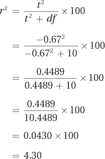
The effect size d, –0.20, is a small effect according to Cohen, while r2 of 4.30% would be classified as a small to medium effect. Why, when we fail to reject the null hypothesis, does there seem to be some effect? There are two explanations for this:
Even if the null hypothesis is true, in which case the size of the effect in the population is zero, it is possible, due to sampling error, that a nonzero effect would be observed in the sample. So, it shouldn’t be surprising to find a small effect.
243
It is also possible that the observed effect size represents the size of the effect in the population. If this were true, it would mean a Type II error is being made.
When a researcher has concern about Type II error, he or she can suggest replication with a larger sample size. A larger sample size has a number of benefits. First, it makes it easier to reject the null hypothesis because a larger sample size, with more degrees of freedom, moves the rare zone closer to the midpoint. It is also easier to reject the null hypothesis because a larger sample makes the standard error of the mean smaller, which makes the t value larger. In fact, if the sample size had been 75 in the pet-loss study, not 11, d would still be –0.20, but the vet would have rejected the null hypothesis.
A statistician would call this study underpowered. To be underpowered means that a study doesn’t include enough cases to have a reasonable chance of detecting an effect that exists. As was mentioned in Chapter 6, if power is low, then beta, the chance of a Type II error, is high. So, raising a concern about one (Type II error) raises a concern about the other (power).
How wide is the confidence interval? The final calculation Dr. Richman should make in order to understand his results is to calculate a 95% confidence interval for the difference between population means. This requires Equation 7.5:
95% CIμDiff = (M – μ) ± (tcv × sM)
= (2.58 – 2.68) ± (2.228 × 0.15)
= –0.1000 ± 0.3342
= from –0.4342 to 0.2342
= from –0.43 to 0.23
Before interpreting this confidence interval, remember that the null hypothesis was not rejected and there is no evidence that pet loss has an effect on GPA. The confidence interval should show this, and it does.
This 95% confidence interval ranges from –0.43 to 0.23. First, note that it includes the value of 0. A value of 0 indicates no difference between the two population means and so it is a possibility, like the null hypothesis said, that there is no difference between the two populations. The confidence interval for the difference between population means should capture zero whenever the null hypothesis is not rejected. (This is true for a 95% confidence interval as long as the hypothesis test is two-tailed with α = .05.)
Next, Dr. Richman looks at the upper and lower ends of the confidence interval, –0.43 and 0.23. This confidence interval tells him that it is possible the average GPA for the population of students who have lost a pet could be as low as 0.43 points worse than the general student average, or as high as 0.23 points better than the general student average. This doesn’t provide much information about the effect of pet loss on academic performance—maybe it helps, maybe it hurts.
Finally, he looks at the width of the confidence interval using Equation 7.6:
CIW = CIUL – CILL
= 0.23 – (–0.43)
= 0.23 + 0.43
= 0.6600
= 0.66
244
The confidence interval is 0.66 points wide. This is a fairly wide confidence interval for a variable like GPA, a variable that has a maximum range of 4 points.
A confidence interval is better when it is narrower, because a narrower one gives a more precise estimate of the population value. How does a researcher narrow a confidence interval? By increasing sample size. Dr. Richman should recommend replicating with a larger sample size to get a better sense of what the effect of pet loss is in the larger population. Increasing the sample size also increases the power, making it more likely that an effect will be found statistically significant.
Putting it all together. Here’s Dr. Richman’s interpretation. Note that (1) he starts with a brief explanation of the study, (2) reports some facts but doesn’t report everything he calculated, (3) gives his interpretation of the results, and (4) makes suggestions for improving the study.
This study explored whether losing a pet while at college had a negative impact on academic performance. The GPA of 11 students who lost a pet (M = 2.58) was compared to the GPA of the population of students at that college (μ = 2.68). The students who had lost a pet did not have GPAs that were statistically significantly lower [t(10) = –0.67, p > .05 (one-tailed)].
Though there was not sufficient evidence in this study to show that loss of a pet has a negative impact on college performance, the sample size was small and the study did not have enough power to find a small effect. Therefore, it would be advisable to replicate the study with a larger sample size to have a better chance of determining the effect of pet loss and to get a better estimate of the size of the effect.
Practice Problems 7.4
Apply Your Knowledge
7.18 If M = 70, μ = 60, tcv = ±2.086, and sM = 4.36, what is the 95% confidence interval for the difference between population means?
7.19 If M = 55, μ = 50, tcv = ±2.052, and sM = 1.89, what is the 95% confidence interval for the difference between population means?
7.20 A college president has obtained a sample of 81 students at her school. She plans to survey them regarding some potential changes in academic policies. But, first, she wants to make sure that the sample is representative of the school in terms of academic performance. She knows from the registrar that the mean GPA for the entire school is 3.02. She calculates the mean of her sample as 3.16, with a standard deviation of 0.36. She used a single-sample t test to compare the sample mean (3.16) to the population mean (3.02). Using her findings below, determine if the sample is representative of the population in terms of academic performance:
sM = 0.04
t = 3.50
d = 0.39
r2 = 13.28%
95% CIμDiff = from 0.06 to 0.22
Application Demonstration
Chips Ahoy is a great cookie. In 1997 Nabisco came out with a clever advertising campaign, the Chips Ahoy Challenge. Its cookies had so many chocolate chips that Nabisco guaranteed there were more than a thousand chips in every bag. And the company challenged consumers to count. It’s almost two decade later, but do Chips Ahoy cookies still have more than a thousand chocolate chips in every bag? Let’s investigate.
245
It is easier to count the number of chips in a single cookie than to count the number of chips in a whole bag of cookies. If a bag has at least 1,000 chips and there are 36 cookies in a bag, then each cookie should have an average of 27.78 chips. So, here is the challenge rephrased: “Chips Ahoy cookies are so full of chocolate chips that each one contains an average of 27.78 chips. We challenge you to count them.”
Step 1 This challenge calls for a statistical test. The population value is known: μ = 27.78. All that is left is to obtain a sample of cookies; find the sample mean, M; and see if there is a statistically significant difference between M and μ. Unfortunately, Nabisco has not reported σ, the population standard deviation, so the single-sample z test can’t be used. However, it is possible to calculate the standard deviation (s) from a sample, which means the single-sample t test can be used.
Ten cookies were taken from a bag of Chips Ahoy cookies. Each cookie was soaked in cold water, the cookie part washed away, and the chips counted. The cookies contained from 22 to 29 chips, with a mean of 26.10 and a standard deviation of 2.69.
Step 2 The next step is to check the assumptions. The random sample assumption was violated as the sample was not a random sample from the population of Chips Ahoy cookies being manufactured. Perhaps the cookies being manufactured on the day this bag was produced were odd. Given the focus on quality control that a manufacturer like Nabisco maintains, this seems unlikely. So, though this assumption is violated, it still seems reasonable to generalize the results to the larger population of Chips Ahoy cookies.
We’ll operationalize the independence of observations assumption as most researchers do and consider it not violated as no case is in the sample twice and each cookie is assessed individually. Similarly, the normality assumption will be considered not violated under the belief that characteristics controlled by random processes are normally distributed.
Step 3 The hypotheses should be formulated before any data are collected. It seems reasonable to do a nondirectional (two-tailed) test in order to allow for the possibilities of more chips than promised as well as fewer chips than promised. Here are the two hypotheses:
H0: μChips = 27.28
H1: μChips ≠ 27.78
Step 4 The consequences of making a Type I error in this study are not catastrophic, so it seems reasonable to use the traditional alpha level of .05. As already decided, a two-tailed test is being used. Thus, the critical value of t, with 9 degrees of freedom, is ±2.262. Here is the decision rule:
If t ≤ –2.262 or if t ≥ 2.262, reject H0.
If –2.262 < t < 2.262, fail to reject H0.
246
Step 5 The first step in calculating a single-sample t test is to calculate what will be used as the denominator, the estimated standard error of the mean:
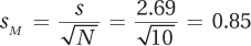
The estimated standard error of the mean is then used to calculate the test statistic, t:
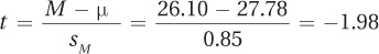
Step 6 The first step in interpreting the results is to determine if the null hypothesis should be rejected. The second statement in the decision rule is true: –2.262 < –1.98 < 2.262, the null hypothesis is not rejected. The difference between 26.10, the mean number of chips found in the cookies, and 27.78, the number of chips expected per cookie, is not statistically significant. From this study, even though the cookies in the bag at M = 26.10 chips per cookie fell short of the expected 27.78 chips per cookie, not enough evidence exists to question Nabisco’s assertion that there are 27.78 chips per cookie and a thousand chips in every bag. And, there’s not enough evidence to suggest that, since 1997, Nabisco’s recipe has changed and/or its quality control has slipped.
Having answered the challenge, it is tempting to stop here. But forging ahead—going on to find Cohen’s d, r2, and the 95% confidence interval—will give additional information and help clarify the results.
Finding Cohen’s d, the size of the effect, provides a different perspective on the results:
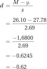
Though the t test says there is not enough evidence to find an effect, Cohen’s d says d = –0.62, a medium effect. This seems contradictory—is there an effect or isn’t there? Perhaps the study doesn’t have enough power and a Type II error is being made. This means that the study should be replicated with a larger sample size before concluding that Chips Ahoy hasn’t failed the thousand chip challenge. Calculating r2 = 30% leads to a similar conclusion.
Does the confidence interval tell a similar story? Here are the calculations for the confidence interval:
95% CIμDiff = (M – μ) ± (tcv × sM)
= (26.10 – 27.78) ± (2.262 × 0.85)
= –1.6800 ± 1.9227
= from –3.6027 to 0.2427
= from –3.60 to 0.24
247
The confidence interval says that the range from –3.60 to 0.24 probably contains the difference between 27.78 (the expected number of chips per cookie) and the number really found in each cookie. As this range captures zero, it is possible that there is no difference, the null hypothesis is true, and bags of cookies really do contain 1,000 chips.
Positive numbers in the confidence interval suggest that the difference lies in the direction of there being more than 27.78 chips per cookie. Negative numbers suggest the difference is in the direction of there being fewer than 27.78 chips per cookie. Most of the confidence interval lies in negative territory. A betting person would wager that the difference is more likely to rest with bags containing fewer than a thousand chips.
The t test left open the possibility that Nabisco still ruled the 1,000 chip challenge. But, thanks to going beyond t, to calculating d and a confidence interval, it no longer seems clear that Nabisco would win the Chips Ahoy challenge. For a complete interpretation of the results of this Chips Ahoy challenge, see Figure 7.11.