CHAPTER EXERCISES
Answers to the odd-numbered exercises appear in Appendix B.
Review Your Knowledge
7.01 In order to use a single-sample t test, one does / does not need to know the population standard deviation.
7.02 The single-sample t test compares a sample ____ to a population ____.
7.03 A sample, selected at random from a population, may have a sample mean that differs from the population mean due to ____.
7.04 Tom ____ Harry ____ ____ infants.
7.05 One assumption of the single-sample t test is that the sample is a random sample from the population. This is / is not robust to violation.
7.06 The population that the sample comes from determines the population to which the results can be ____.
7.07 A second assumption of the single-sample t test is that observations within the sample are ____.
7.08 The third assumption of the single-sample t test is called the ____ assumption for short.
7.09 If a ____ assumption is violated, a researcher can still proceed with the test as long as the violation is not too great.
7.10 In order to write the null and alternative hypotheses for a single-sample t test, the researcher needs to know whether the test has one or two ____.
7.11 The default option in hypothesis testing is a ____-tailed test.
7.12 If a researcher is doing a one-tailed test, he or she should predict the ____ of the results before collecting any data.
7.13 The null hypothesis for a nondirectional, single-sample t test says that the sample does / does not come from the population.
7.14 The null hypothesis for a two-tailed, single-sample t test could be written as ____ = μ2.
7.15 The alternative hypothesis for a two-tailed, single-sample t test could be written as μ1 ____ μ2.
7.16 If the null hypothesis for a two-tailed, single-sample t test is true, t = ____.
7.17 As the distance between the sample mean and the population mean grows, the value of t ____.
250
7.18 he abbreviation for the critical value of t is ____.
7.19 Determining the critical value depends on (a) how many ____ the test has, (b) how willing one is to make a Type ____ error, and (c) the ____.
7.20 If the hypotheses are nondirectional, then the researcher is doing a ____-tailed test.
7.21 If the alternative hypothesis is μ > 173, then the test is a ____-tailed test.
7.22 If the researcher wants a 5% chance of Type I error, then alpha is set at ____.
7.23 For a two-tailed test with α = .05, the rare zone has ____% of the sampling distribution in each tail.
7.24 When the sample size is large, the rare zone gets ____ and it is ____ to reject the null hypothesis.
7.25 Degrees of freedom, for a single-sample t test, equal ____ minus 1.
7.26 For a two-tailed, single-sample t test, the null hypothesis is rejected if t ≤ ____ or if t ≥ ____.
7.27 t for a single-sample t test is calculated by dividing the difference between M and μ by ____.
7.28 Interpretation uses human ____ to make meaning out of the results.
7.29 Interpretation is subjective, but needs to be supported by ____.
7.30 The first question asked in interpretation is about whether the ____ hypothesis is ____.
7.31 For the second interpretation question, one calculates ____, and for the third, one calculates a ____.
7.32 A decision is made about rejecting the null hypothesis by comparing the ____ value of t to the value calculated from the sample mean.
7.33 If a researcher rejects the null hypothesis, then he or she is forced to accept the ____.
7.34 If the null hypothesis is rejected, it is concluded that the mean for the population the ____ came from differs from the hypothesized value.
7.35 To determine the direction of a statistically significant difference, compare the ____ to the ____.
7.36 Sample size is reported in APA format for a single-sample t test by reporting ____.
7.37 APA format uses the inequality ____ to indicate that the null hypothesis was rejected when α = .05.
7.38 If a result is reported in APA format as p < .05, that means the observed value of the test statistic fell in the ____ zone.
7.39 If one fails to reject the null hypothesis, one can say that there is ____ to conclude a difference exists between the population means.
7.40 APA format uses the inequality ____ to indicate that the null hypothesis was not rejected when α = .05.
7.41 Effect sizes are used to quantify the impact of the ____ on the ____.
7.42 Cohen’s d is an ____.
7.43 A value of 0 for Cohen’s d means that the independent variable had ____ impact on the dependent variable.
7.44 Cohen considers a d of ____ a small effect, ____ a medium effect, and ____ or higher a large effect.
7.45 As the effect size d increases, the degree of overlap between the distributions for two populations ____.
7.46 When one fails to reject the null hypothesis, one should ____ calculate Cohen’s d.
7.47 Calculating d when one has failed to reject the null hypothesis alerts one to the possibility of a Type ____ error.
7.48 To ____ a study is to repeat it.
7.49 r2 measures how much variability in the _____ is explained by the _______.
7.50 d and r2 should lead to similar conclusions about the size of an effect. Though both may have been calculated, it is _____ to report both.
251
7.51 If a researcher calculates a 95% confidence interval, he or she can be ____% confident that it captures the ____ value.
7.52 The 95% confidence interval for the difference between population means tells how far apart or how close the two ____ means might be.
7.53 The size of the difference between population means can be thought of as another ____.
7.54 If a 95% confidence interval for the difference between population means does not capture zero, and the researcher is doing a two-tailed test with α = .05, then the null hypothesis was / was not rejected.
7.55 If the 95% confidence interval for the difference between population means falls close to zero, this means the size of the effect may be ____.
7.56 A wide 95% confidence interval for the difference between population means leaves a researcher unsure of ____.
Apply Your Knowledge
Picking the right test
7.57 A researcher has a sample (N = 38, M = 35, s = 7) that he thinks came from a population where μ = 42. What statistical test should he use?
7.58 A researcher has a sample (N = 52, M = 17, s = 3) that she believes came from a population where μ = 20 and σ = 4. What statistical test should she use?
Checking the assumptions
7.59 A researcher wants to compare the mean weight of a convenience sample of students from a college to the national mean weight of 18- to 22-year-olds. (a) Check the assumptions and decide whether it is OK to proceed with a single-sample t test. (b) Can the researcher generalize the results to all the students at the college?
7.60 There is a random sample of students from a large public high school. Each person, individually, takes a paper-and-pencil measure of introversion. (a) Check the assumptions and decide whether it is OK to proceed with a single-sample t test to compare the sample mean to the population mean of introversion for U.S. teenagers. (b) To what population can one generalize the results? (The same introversion measure was used for the national sample.)
Writing nondirectional hypotheses
7.61 The population mean on a test of paranoia is 25. A psychologist obtained a random sample of nuns and found M = 22. Write the null and alternative hypotheses.
7.62 A researcher wants to compare a random sample of left-handed people in terms of IQ to the population mean of IQ. Given M = 108 and assuming μ = 100, write the null and alternative hypotheses.
Writing directional hypotheses
7.63 In America, the average length of time the flu lasts is 6.30 days. An infectious disease physician has developed a treatment that he believes will treat the flu more quickly. Write the null and alternative hypotheses.
7.64 An SAT-tutoring company claims that its students perform above the national average on SAT subtests. If the national average on SAT subtests is 500 and the tutoring company obtains SAT scores from a random sample of 626 of its students, write the null and alternative hypotheses.
Finding tcv (assume the test is two-tailed and alpha is set at .05)
7.65 If N = 17, find tcv and use it to draw a t distribution with the rare and common zones labeled.
7.66 If N = 48, find tcv and use it to draw a t distribution with the rare and common zones labeled.
Writing the decision rule (assume the test is two-tailed and alpha is set at .05)
7.67 If N = 64, write the decision rules for a single-sample t test.
252
7.68 If N = 56, write the decision rules for a single-sample t test.
Calculating sM
7.69 If N = 23 and s = 12, calculate sM.
7.70 If N = 44 and s = 7, calculate sM.
Given sM, calculating t
7.71 If M = 10, μ = 12, and sM = 1.25, what is t?
7.72 If M = 8, μ = 6, and sM = 0.68, what is t?
Calculating t
7.73 If N = 18, M = 12, μ = 10, and s = 1, what is t?
7.74 If N = 25, M = 18, μ = 13, and s = 2, what is t?
Was the null hypothesis rejected? (Assume the test is two-tailed.)
7.75 If tcv = ±2.012 and t = –8.31, is the null hypothesis rejected?
7.76 If tcv = ±2.030 and t = 2.16, is the null hypothesis rejected?
7.77 If tcv = ±2.776 and t = 1.12, is the null hypothesis rejected?
7.78 If tcv = ±1.984 and t = –1.00, is the null hypothesis rejected?
Writing results in APA format (Assume the test is two-tailed and alpha is set at .05.)
7.79 Given N = 15 and t = 2.145, write the results in APA format.
7.80 Given N = 28 and t = 2.050, write the results in APA format.
7.81 Given N = 69 and t = 1.992, write the results in APA format.
7.82 Given N = 84 and t = 1.998, write the results in APA format.
Calculating Cohen’s d
7.83 Given M = 90, μ = 100, and s = 15, calculate Cohen’s d.
7.84 Given M = 98, μ = 100, and s = 15, calculate Cohen’s d.
Calculating r2
7.85 Given N = 17 and t = 3.45, what is r2?
7.86 If N = 29 and t = 1.64, what is r2?
Calculating a 95% confidence interval
7.87 Given M = 45, μ = 50, tcv = ±2.093, and sM = 2.24, calculate the 95% confidence interval for the difference between population means.
7.88 Given M = 55, μ = 50, tcv = ±2.093, and sM = 2.24, calculate the 95% confidence interval for the difference between population means.
Given effect size and confidence interval, interpret the results. Be sure to (1) tell what was done, (2) present some facts, (3) interpret the results, and (4) make a suggestion for future research. (Assume the test is two-tailed and α = .05.)
7.89 Given the supplied information, interpret the results. A nurse practitioner has compared the blood pressure of a sample (N = 24) of people who are heavy salt users (M = 138, s = 16) to blood pressure in the general population (μ = 120) to see if high salt consumption were related to raised or lowered blood pressure. She found:
tcv = 2.069
t = 5.50
d = 1.13
r2 = 57%
95% CI [11.23, 24.77]
7.90 Given the supplied information, interpret the results. A dean compared the GPA of a sample (N = 20) of students who spent more than two hours a night on homework (M =3.20, s = 0.50) to the average GPA at her college (μ = 2.80). She was curious if homework had any relationship, either positive or negative, with GPA. She found:
tcv = 2.093
t = 3.64
d = 0.80
r2 = 41%
95% CI [0.17, 0.63]
Completing all six steps of a hypothesis test
7.91 An educational psychologist was interested in time management by students. She had a theory that students who did well in school spent less time involved with online social media. She found out, from the American Social Media Research Collective, that the average American high school student spends 18.68 hours per week using online social media. She then obtained a sample of 31 students, each of whom had been named the valedictorian of his or her high school. These valedictorians spent an average of 16.24 hours using online social media every week. Their standard deviation was 6.80. Complete the analyses and write a paragraph of interpretation.
253
7.92 A psychology professor was curious how psychology majors fared economically compared to business majors. Did they do better, or did they do worse five years after graduation? She did some research and learned that the national mean for the salary of business majors five years after graduation was $55,000. She surveyed 22 recent psychology graduates at her school and found M = $43,000, s = 12,000. Complete the analyses and write a paragraph of interpretation.
Expand Your Knowledge
7.93 Imagine a researcher has taken two random samples from two populations (A and B). Each sample is the same size (N = 71), has the same sample mean (M = 50), and comes from a population with the same mean (μ = 52). The two populations differ in how much variability exists. As a result, one sample has a smaller standard deviation (s = 2) than the other (s = 12). The researcher went on to calculate single-sample t values for each sample. Based on the information provided below, how does the size of the sample standard deviation affect the results of a single-sample t test?
| sM | tcv | t | d | r2 | CI | Width of CI | |
| A: Less variability (s = 2) | 0.24 | 1.994 | –8.33 | –1.00 | 50% | –2.48 to –1.52 | 0.96 |
| B: More variability (s = 12) | 1.42 | 1.994 | –1.41 | –0.17 | 3% | –4.83 to 0.83 | 5.66 |
7.94 Another researcher selected two random samples from one population. This population has a mean of 63 (μ = 63). It turned out that each sample had the same mean (M = 60) and standard deviation (s = 5). The only way the two samples differed was in terms of size: one, C, was smaller (N = 10) and one, D, was larger (N = 50). The researcher went on to conduct a single-sample t test for each sample. Based on the information provided below, how does sample size affect the results of a single-sample t test?
| sM | tcv | t | d | r2 | CI | Width of CI | |
| C: Smaller N (N = 10) | 1.58 | 2.262 | –1.90 | –0.60 | 29% | 6.57 to 0.57 | 7.14 |
| D: Larger N (N = 50) | 0.71 | 2.010 | –4.23 | –0.60 | 27% | 4.43 to –1.57 | 2.86 |
7.95 A third researcher obtained two random samples from another population. The mean for this population is 50 (μ = 50). Each sample was the same size (N = 10) and each had the same standard deviation (s = 20). But one, sample E, had a mean of 80 (M = 80) and the other, sample F, a mean of 60 (M = 60). Based on the information provided below, how does the distance from the sample mean to the population mean affect the results of a single-sample t test?
| sM | tcv | t | d | r2 | CI | Width of CI | |
| E: M farther from μ(M = 80) | 6.32 | 2.262 | 4.75 | 1.50 | 71% | 15.70 to 44.30 | 28.60 |
| F: M closer to μ(M = 60) | 6.32 | 2.262 | 1.58 | 0.50 | 22% | –4.30 to 24.30 | 28.60 |
7.96 Based on the answers to Exercises 7.93 to 7.95, what factors have an impact on a researcher’s ability to reject the null hypothesis? Which one(s) can he or she control?
7.97 A researcher is conducting a two-tailed, single-sample t test with alpha set at .05. What is the largest value of t that one could have that, no matter how big N is, will guarantee failing to reject the null hypothesis?
254
7.98 If tcv for a two-tailed test with α = .05 is ±2.228, what would the alpha level be for the critical value of 2.228 as a one-tailed test?
7.99 If N = 21 and sM = 1, write as much of the equation as possible for calculating the 90% CIμDiff and the 99% CIμDiff. Use Equation 7.4 as a guide.
7.100 Which confidence interval in Exercise 7.95 is wider: 90% or 99%? Explain why.
SPSS
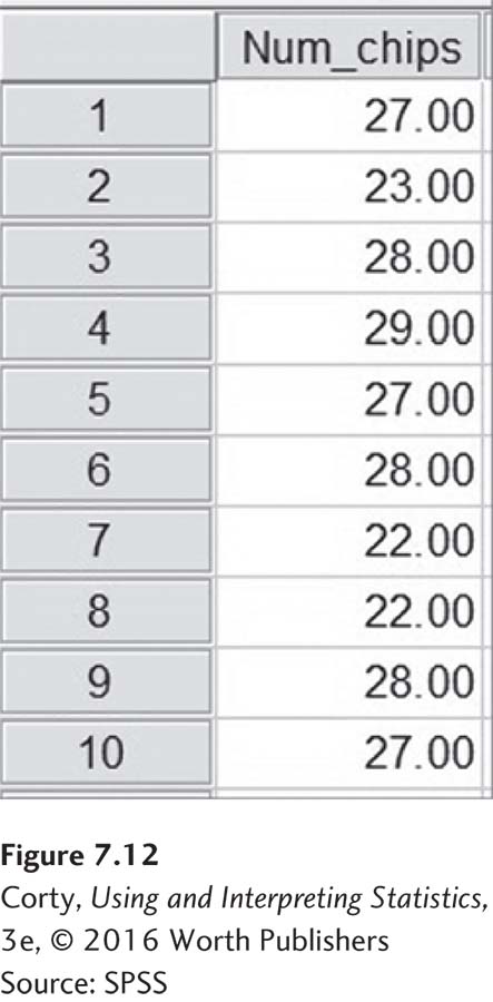
Let’s use SPSS to analyze the Chips Ahoy data from the Application Demonstration at the end of the chapter. The first step is data entry. Figure 7.12 shows the data for the 10 cookies. Note that the variable is labeled “Num_chips” at the top of the column, and that the value for each case appears in a separate row.
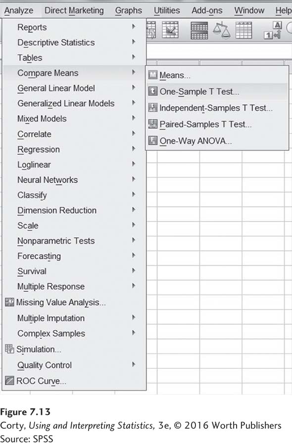
SPSS calls a single-sample t test the “One-Sample T Test.” It is found by clicking on “Analyze” on the top line (Figure 7.13). Then click on “Compare Means” and “One-Sample T Test. . . .”
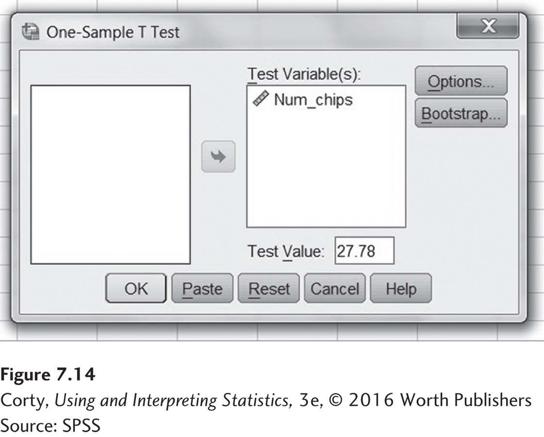
This pulls up the box seen in Figure 7.14. Note that the variable “Num_chips,” which we wish to analyze, has already been moved over from the box on the left (which is now empty) to the box labeled “Test Variable(s).” The population mean, 27.78, has been entered into the box labeled “Test Value.” Once this is done, it is time to click the “OK” button on the lower right.
255
Figure 7.15 shows the output that SPSS produces. There are a number of things to note:
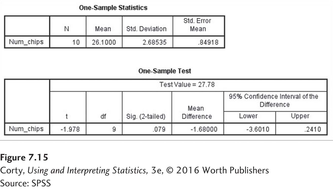
The first box provides descriptive statistics, including the standard error of the mean, sM, the denominator for t.
At the top of the second output box, “Test Value = 27.78” indicates that this is the value against which the sample mean is being compared.
Next, SPSS reports the t value (–1.978) and the degrees of freedom (9).
SPSS then reports what it calls “Sig. (2-tailed)” as .079.
The important thing for us is whether this value is ≤ .05 or > .05.
If it is ≤ .05, the null hypothesis is rejected and the results are reported in APA format as p < .05.
If it is > .05, the null hypothesis is not rejected and the results are reported in APA format as p > .05.
This value, .079, is the exact significance level for this test with these data. It indicates what the two-tailed probability is of obtaining a t value of –1.978 or larger if the null hypothesis is true. In the present situation, it says that a t value of –1.978 is a common one—it happens 7.9% of the time when 10 cases are sampled from a population where μ = 27.78. APA format calls for the exact significance level to be used. Thus, these results should be reported as t (9) = –1.98, p = .079.
The next bit of output reports the mean difference, –1.68, between the sample mean (26.10) and the test value (27.78).
SPSS reports what it calls the “95% Confidence Interval of the Difference,” what is called in the book the 95% confidence interval for the difference between population means, ranging from a “Lower” bound of –3.60 to an “Upper” bound of 0.24.
Note that SPSS does not report Cohen’s d. Similarly, there is not enough information to calculate r2. However, it provides enough information, the mean difference (–1.68) and the standard deviation (2.685), that it can be done by hand with Equation 7.3.