9.2 Calculating the Paired-Samples t Test
Here are some data that are appropriate for analysis with a paired-samples t test. Imagine that a sensory psychologist, Dr. Keim, wanted to examine the effect of humidity on perceived temperature. She obtained six volunteers at her college and tested them, individually, in a temperature- and humidity-controlled chamber. Each participant was tested twice and the tests were separated by 24 hours. For both tests, the temperature in the chamber was set at 76°F. For one test the humidity level was “low,” and for the other test the humidity level was “high.” In order to avoid any effects due to the order of the tests, which humidity level each participant would experience first was randomly determined. For a test, a participant spent 15 minutes in the chamber, after which he or she was asked what the temperature was inside it. This “perceived temperature” is the study’s dependent variable.
The data from the humidity study are shown in Table 9.1, where each case appears on a row and each condition (sample) in a column. Table 9.1 also contains the means and standard deviations for both conditions. Remember, in both conditions the actual temperature was the same, 76°F. The mean perceived temperature on the low-humidity test was 75.00°F, and in the high-humidity condition it was 82.50°F. Between the two test conditions, there was a 7.50°F difference in the means.
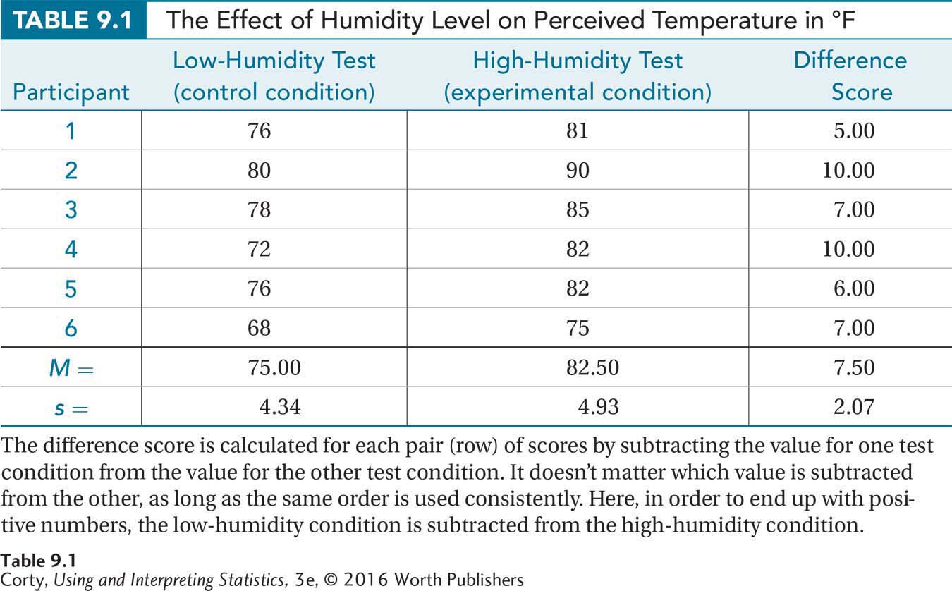
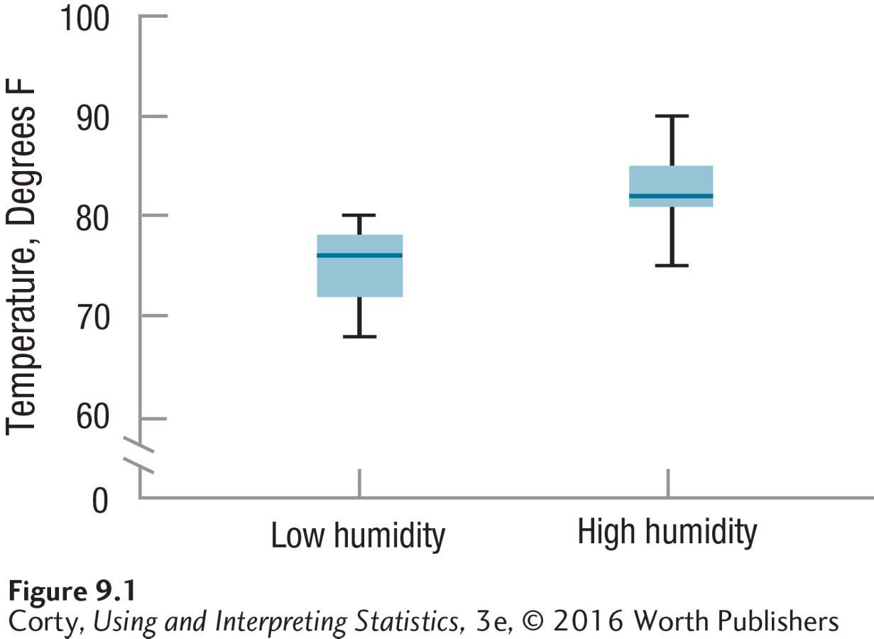
Figure 9.1 is a pair of box-and-whisker plots, showing the median, interquartile range, and minimum/maximum for each condition. When looking at the graph, the difference seems clear—temperature does appear to be perceived as higher when the humidity is higher. But, looks can be deceiving and the sample size is low, so hypothesis testing is necessary to find out if the difference is a statistically significant one or if it can be explained by sampling error.
Step 1 Pick a Test. Dr. Keim, using a within-subjects design, is comparing the means for a sample of people measured in two different conditions, low humidity and high humidity. Remember, when one sample is measured in two different conditions, as happens here, statisticians consider this two dependent samples. This situation, comparing the means of dependent samples, calls for a paired-samples t test.
296
Step 2 Check the Assumptions. There are three assumptions for the paired-samples t test (Table 9.2), and they are familiar. The first assumption is that the sample is a random sample from the population to which the results will be generalized. Dr. Keim would like to be able to generalize her results to people in general, that is, to all the people in the world. She recognizes that she has a convenience sample not a random sample from this population, so this assumption is violated. The random samples assumption is robust, however, so she can continue with the test. She is aware of no one who suggests that Americans and/or college students perceive heat differently from others, so she will be willing to generalize her results more broadly than just to U.S. college students.
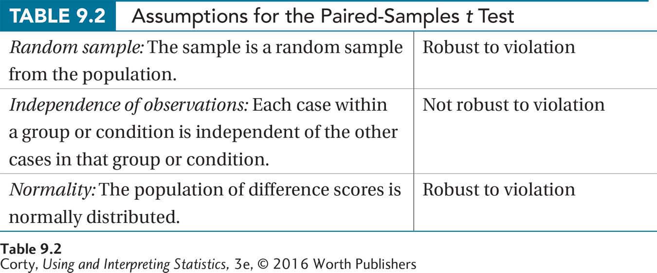
The second assumption is that the observations are independent within a sample. Be careful in assessing this assumption: it refers to independence within a sample, not between samples. Since the same cases are in both samples, or conditions, the two samples are not independent. However, each person in each sample is tested individually and each person is only tested once in each condition. The independence of observations assumption is not violated.
297
The third assumption, the normality assumption, says that in the larger population the difference scores are normally distributed. Look at Table 9.1 and note that there’s a third column listing the difference between the value a case had in one condition (high humidity) and its score in the other condition (low humidity). This is called a difference score, abbreviated D, and is needed to calculate a paired-samples t test. The formula for D is shown in Equation 9.1.
Equation 9.1 Formula for Calculating Difference Score, D
D = X1 – X2
where D = the difference score being calculated
X1 = a case’s score in Condition 1
X2 = a case’s score in Condition 2
In calculating D, it matters little which value is subtracted from the other, as long as the same order is followed for all cases. Most people prefer to work with positive numbers, so feel free to decide the order for the subtraction to maximize the number of positive values. Dr. Keim chose to subtract the low-humidity scores from the high-humidity scores in order to have positive difference scores.
For the first case, the person who perceived the low-humidity condition as 76° and the high-humidity condition as 81°F, the difference score is calculated as
D = XHighHumidity – XLowHumidity
= 81 – 76
= 5.0000
= 5.00
A sample size of 6 is a little small for making decisions about the shape of a parent population. However, based on her previous research, Dr. Keim is willing to assume that the difference scores are normally distributed in the population, so the normality assumption is not violated.
Step 3 List the Hypotheses. The hypotheses, which are statements about populations, are going to be the same as they were for the independent-samples t test. The null hypothesis is going to say that the two population means are the same. The alternative hypothesis will state that the two population means differ, but it won’t indicate whether the difference is large or small, positive or negative. These hypotheses are nondirectional or two-tailed, so they don’t specify a direction for the difference. Thus, Dr. Keim is testing for two possibilities: (1) low humidity is perceived as hotter than high humidity, or (2) high humidity is perceived as hotter than low humidity. The generic form of two-tailed hypotheses is
298
H0: µ1 = µ2
H1: µ1 ≠ µ2
The specific form of the two hypotheses for this study is
H0: µLowHumidity = µHighHumidity
H1: µLowHumidity ≠ µHighHumidity
Of course, it is possible to have directional hypotheses for a paired-samples t test. If Dr. Keim had predicted, in advance, that high humidity would lead to a higher perceived temperature, her hypotheses would have been
H0: µLowHumidity ≥ µHighHumidity
H1: µLowHumidity < µHighHumidity
Step 4 Set the Decision Rule. The decision rule for a paired-samples t test is formulated the same way as it was for the independent-samples t test. The critical value of t, tcv , found in Appendix Table 3, is based on (1) the number of tails for the test, (2) how willing one is to make a Type I error (i.e., the alpha level), and (3) how many degrees of freedom there are. The default option, or the most common form of the paired-samples t test, as for other statistical tests, is a two-tailed test with alpha set at .05.
Once the observed value of t is calculated (Step 5), it is compared to the critical value in order to decide whether or not to reject the null hypothesis. For a two-tailed test, the general form of the decision rule is:
If t ≤ –tcv or t ≥ tcv , reject the null hypothesis.
If –tcv < t < tcv , fail to reject the null hypothesis.
Dr. Keim is doing a two-tailed test and is content to use the default alpha level of .05. All that she needs to do is calculate degrees of freedom. Equation 9.2 is the formula for calculating degrees of freedom for a paired-samples t test.
Equation 9.2 Degrees of Freedom (df) for a Paired-Samples t Test
df = N – 1
where df = the degrees of freedom
N = the number of pairs of cases
Dr. Keim’s study involves six pairs of cases, so degrees of freedom are calculated as
df = 6 – 1
= 5
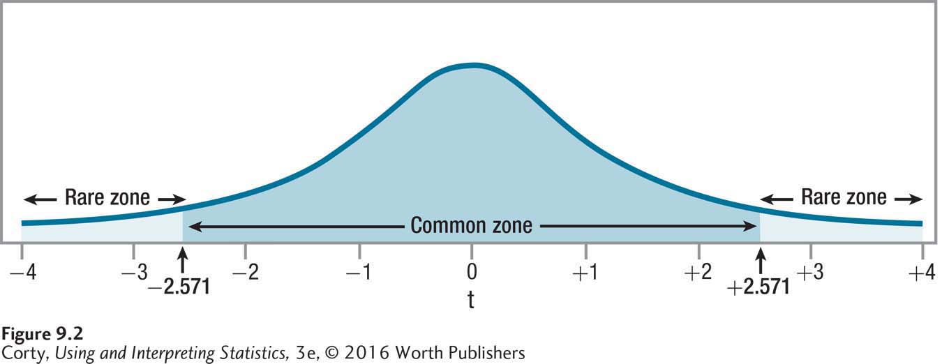
Look in Appendix 3 and find the intersection of the column for a two-tailed hypothesis test with the alpha set at .05 and the row for df = 5. There, the critical value of t, ±2.571, is found. Figure 9.2 uses the critical values to mark the rare zone, where the null hypothesis is rejected, and the common zone, where it is not.
299
Here is the decision rule for Dr. Keim’s study:
If t ≤ –2.571 or t ≥ 2.571, reject the null hypothesis.
If –2.571 < t < 2.571, fail to reject the null hypothesis.
Step 5 Calculate the Test Statistic. The same general procedure is used for calculating the paired-samples t value as was used for the independent-samples t: divide the difference between the two sample means by the standard error of the difference. This standard error of the difference is the standard error of the difference for difference scores and will be abbreviated  to differentiate it from the other denominators for t tests. The standard error of the mean difference for difference scores is the standard deviation of the sampling distribution of difference scores.
Equation 9.3 Formula for the Standard Error of the Mean Difference for Difference Scores (sMD)
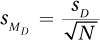

sD = the standard deviation (s) of the difference scores
N = the number of pairs of cases
Using Equations 3.6 and 3.7, Dr. Keim has calculated the standard deviation of the difference scores and found sD = 2.07. There are six pairs of cases, so N = 6. Plugging these values into Equation 9.3 gives
300
The standard error of the mean difference for the difference scores is 0.85. This value will be used in Equation 9.4, the formula for calculating t, the value of the test statistic for the paired-samples t test.
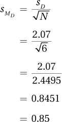
Equation 9.4 Formula for Calculating t, the Value of the Test Statistic for a Paired-Samples t Test
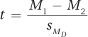
where t = the value of the test statistic for a paired-samples t test
M1 = the mean of one sample
M2 = the mean of the other sample
= standard error of the mean difference for difference scores (Equation 9.3)
Given  , MLowHumidity = 75.00, and MHighHumidity = 82.50, Dr. Keim is ready to calculate t. Again, it matters little which mean is called M1 and which is M2, so Dr. Keim has arranged the calculations to end up with a positive number in the numerator, assuring a positive t value:
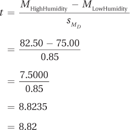
Dr. Keim’s t value is 8.82, and she is done with Step 5. In the next section of the chapter, after more practice with the first five steps, we’ll follow Dr. Keim as she applies the decision rule and interprets the results.
Worked Example 9.1
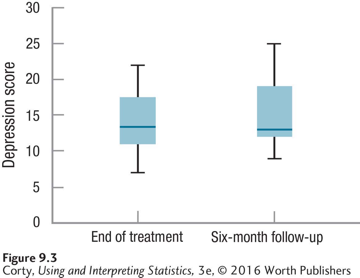
A clinical psychologist, Dr. Althof, was studying the long-term effectiveness of psychodynamic psychotherapy for depression. He obtained a sample of 16 people with moderate to severe depression and assigned each to receive 20 sessions of psychodynamic therapy from a trained therapist. At the end of treatment, he administered a depression scale to each person and determined that the mean level of depression was 14.00. Scores on this depression scale can range from 0 to 50, and higher scores indicate greater depression. Six months later, Dr. Althof tracked down all 16 participants and readministered the depression scale, finding the mean was now 15.00. Figure 9.3 is a pair of box-and-whisker plots showing the depression scores at the two points in time. A 1-point increase on a 50-point scale doesn’t sound like very much, but the box-and-whisker plots suggest an increase in the depression level in the six months following the end of treatment. Dr. Althof needs hypothesis testing to find out if the change is a statistically significant one.
301
Step 1 Pick a Test. Dr. Althof is comparing the mean of a sample at one time to the mean of the sample at a second time. Though it is one sample of people, they are measured at two points in time, making it appropriate for a paired-samples t test.
Step 2 Check the Assumptions. The assumptions for the paired-samples t test are listed in Table 9.2.
The random samples assumption is violated. It is not reported that the 16 cases were a random sample from the population of all the people in the world with moderate to severe depression, so it is safe to assume this is not a random sample from that population. When this robust assumption is violated, however, a researcher can still proceed with the test. Dr. Althof just has to be careful about the population to which he generalizes the results.
The independence of observations assumption is not violated. Each participant received individual therapy, so the participants within a sample didn’t influence each other.
The assumption for the normality of difference scores is not violated. Dr. Althof knows from his review of the literature that depression scores are normally distributed. He is willing to assume that the difference scores (six-month follow-up depression score minus end-of-treatment depression score) will be normally distributed in the larger population.
Step 3 List the Hypotheses. Sometimes the effect of treatment increases over time, but more often the effect of treatment decreases over time, so Dr. Althof was open to both options when he planned the study. As a result, his hypotheses are nondirectional (two-tailed). The null hypothesis states that the two population means (end-of-treatment mean vs. six-month follow-up mean) are the same, and the alternative hypothesis says that the two population means differ:
H0: µEOT = µ6MFU
H1: µEOT ≠ µ6MFU
302
Step 4 Set the Decision Rule. The critical value of t depends on the number of tails, alpha, and degrees of freedom. With nondirectional hypotheses, the test is two-tailed. Dr. Althof is comfortable setting the alpha at the usual level, .05, and having a 5% chance of Type I error. Finally, using Equation 9.2, he calculates degrees of freedom for the paired-samples t test:
df = N – 1
= 16 – 1
= 15
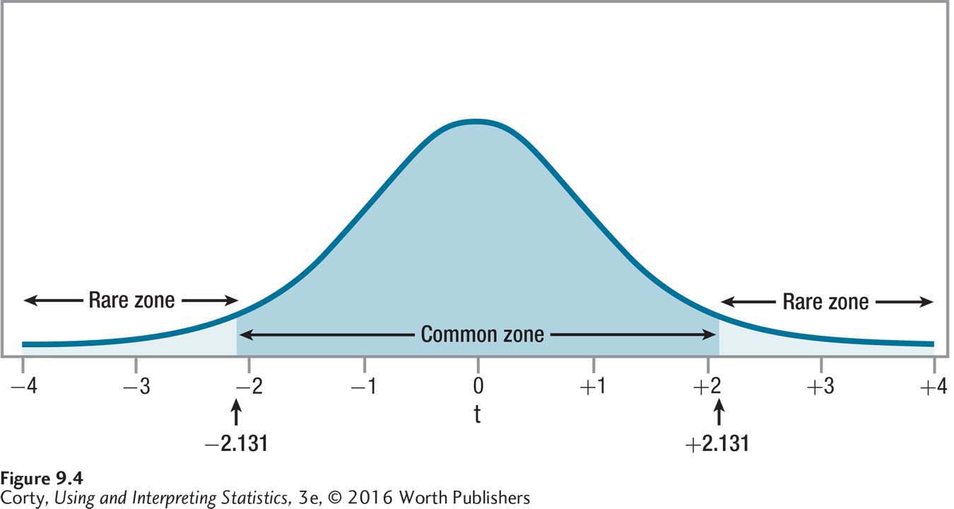
Consulting Appendix Table 3 in the column for a two-tailed test with an alpha of .05 and the row with 15 degrees of freedom, Dr. Althof finds that the critical value of t is ±2.131. The common and rare zones for his decision rule are shown in Figure 9.4. The decision rule is:
If t ≤ –2.131 or t ≥ 2.131, reject the null hypothesis.
If –2.131 < t < 2.131, fail to reject the null hypothesis.
Step 5 Calculate the Test Statistic. The data set, with depression scores at the end of treatment and six months later, is shown in Table 9.3. Also shown are the difference scores and the standard deviation of the difference scores (sD = 2.31).
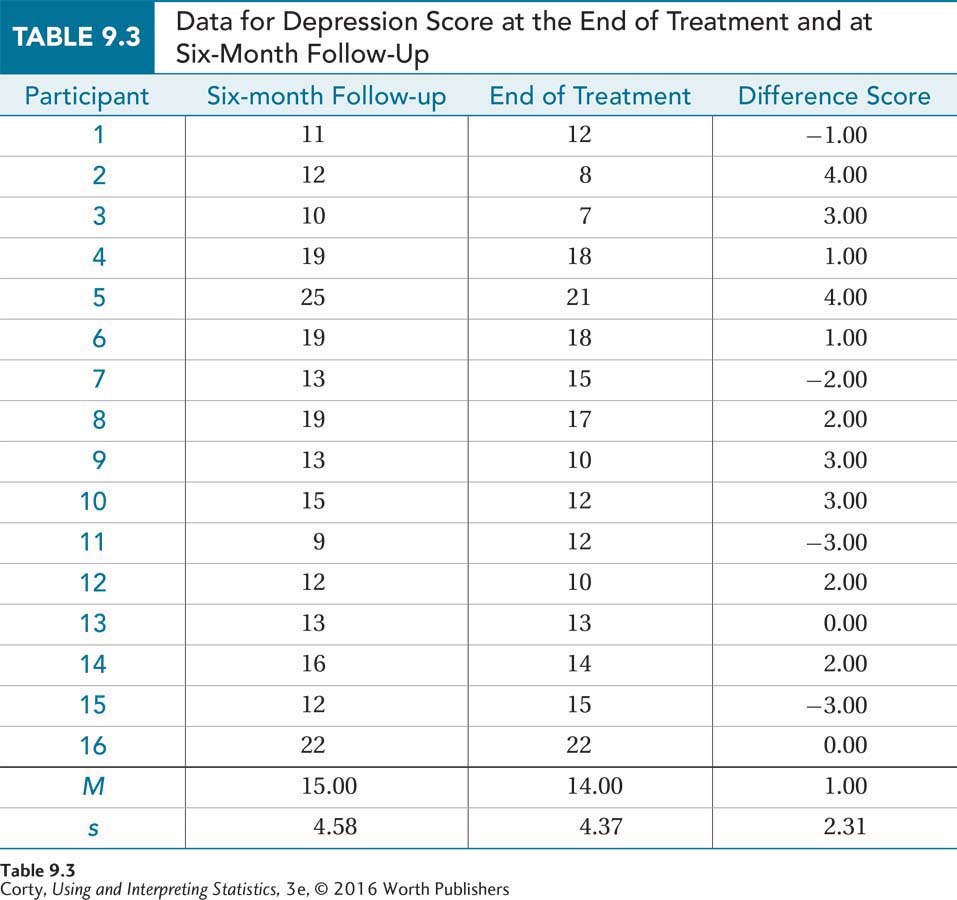
The first step in the calculations is applying Equation 9.3 to find the standard error of the difference, :
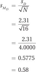
The value for the standard error of the difference, 0.58, is then used in Equation 9.4 to find t. It doesn’t matter which mean is subtracted from which, so Dr. Althof arranged them to end up with a positive value by subtracting the follow-up mean (14.00) from the end-of-treatment mean (15.00):
303
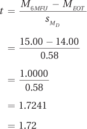
Having found t = 1.72, Step 5 is complete. All that’s left is the interpretation, which we’ll turn to in the next section.
Practice Problems 9.1
Apply Your Knowledge
9.01 Given the following pairs of scores, calculate difference scores: 72 and 75; 69 and 45; 42 and 39; 47 and 46; 55 and 61; 50 and 61; 71 and 69; 55 and 69.
9.02 Given sD = 8.43 and N = 64, calculate .
9.03 Given M1 = 19.98, M2 = 18.65, and  , calculate t.