The Quantity Theory of Money
We already have a good idea about the causes of inflation from the opening discussion of Zimbabwe. We can now examine the inflationary mechanism in more detail by explaining the quantity theory of money. The quantity theory of money does two things: First, it sets out the general relationship between money, velocity (to be defined soon), real output, and prices; second, it helps to explain the critical role of the money supply in determining the inflation rate.
Imagine that every month you are paid $4,000 and you spend $4,000. In a year, you spend $4,000 12 times, so your total yearly spending is $4,000 × 12 = $48,000. Another way of figuring out your total yearly spending is to add up all the goods that you buy and multiply by their prices. We can write this identity (an equation that must hold true by definition) as
254
M × v = P × YR
v, velocity of money, is the average number of times a dollar is spent on final goods and services in a year.
where M is the money you are paid, v is the number of times in a year that you spend M (we call v the “velocity of money,” hence the v), P is prices, and YR is a measure of the real goods and services that you buy. A similar identity holds for the nation as a whole, where we interpret M as the supply of money, v as the average number of times in a year that a dollar is spent on final goods and services, P as the price level, and YR as real GDP.
Thus, for the nation as a whole, we can write
Mv = PYR
|
M = Money supply |
P = Price level |
|
v = Velocity of money |
YR = Real GDP |
Since Mv is the total amount spent on final goods and services and PYR is the price level times real GDP, both sides of this equation are also equal to nominal GDP.
With some additional assumptions, the simple identity, Mv = PYR, helps us think through how money affects output and prices. We proceed with two further assumptions, namely that both real GDP (YR) and velocity (v) are stable compared to the money supply (M).
255
Let’s discuss why these assumptions are usually reasonable. Over the period we are interested in, real GDP is fixed by the real factors of production—capital, labor, and technology—exactly as discussed in Chapter 27 and Chapter 28 on growth. We know that inflation can be 10%, 500%, 5,000% a year, or much higher. Real GDP, in contrast, never grows by more than, say, 10% a year (and that is extraordinary performance), so changes in real GDP don’t seem like a plausible candidate for explaining large changes in prices.
Let’s also assume that v, the velocity of money, is stable. The velocity of money is the average number of times a dollar is used to purchase final goods and services within a year. In the preceding example, v was 12 because you were paid monthly and you spent your entire monthly income of $4,000, 12 times in a year. In the U.S. economy today, v is about 7 and it is determined by the same kind of factors that might determine your personal v, factors such as whether workers are paid monthly or biweekly, how long it takes to clear a check, and how easy it is to find and use an ATM. These factors change over time but only slowly. Other factors that we will discuss at greater length in the chapters on business fluctuations can change v more quickly, but not by enough to account for large and sustained increases in prices. For these reasons, changes in v also do not seem like a plausible candidate for explaining large and sustained increases in prices.
The Cause of Inflation
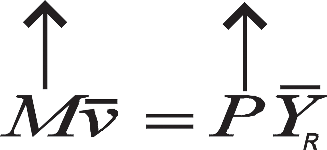
The Quantity Theory of Money in a Nutshell When v and Y are fixed (indicated by a top bar), increases in M must cause increases in P.
If YR is fixed by the real factors of production and v is stable, then it follows immediately that the only thing that can cause increases in P are increases in M, the supply of money. In other words, inflation is caused by an increase in the supply of money.
How well does this theory hold up? The left panel of Figure 31.4 plots the price level (P) and the supply of money (M) in Peru during its hyperinflation. A product with a price of 1 Peruvian intis in 1980 would have cost more than 10 million intis by 1995. (To reduce the number of zeroes, the Peruvian government changed the name of the currency twice during this period, first from intis to soles de oro and then to the nuevo sol.) As you can see, the supply of money also increased about 10 million times in lockstep with the increase in prices.

256
The quantity theory of money can also be written in terms of growth rates. We denote the growth rate of any variable with a little arrow over the variable, so  is the growth rate of the money supply,
  is the growth rate of prices, and so forth. If Mv = PYR, then it is also true that:*
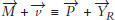
We have a special word for the growth rate of prices : inflation! (Inflation is also often written with a special symbol, π.) If we assume that velocity isn’t changing much, as we just did, then the growth rate of velocity  will be zero or very low. We also know that
  , the growth rate of real GDP, is relatively low, say, between 2% and at most 10%. Thus, if we ignore these two factors, we see immediately that ≈ Inflation Rate (π), where ≈ means approximately equal. In other words, the quantity theory of money says that the growth rate of the money supply will be approximately equal to the inflation rate.
The right panel of Figure 31.4 shows that during Peru’s hyperinflation, this was true: As the supply of money grew faster, so did the inflation rate, peaking in 1990 at a rate of 7,500% per year.
What about other times and places? Figure 31.5 plots inflation rates on the vertical axis versus money growth rates on the horizontal axis for 110 nations between 1960 and 1990. Nations with rapidly growing money supplies had high inflation rates. Nations with slowly growing money supplies had low inflation rates. In fact, as the red line indicates, on average, the relationship is almost perfectly linear, with a 10 percentage point increase in the money growth rate leading to a 10 percentage point increase in the inflation rate.

If we are thinking about sustained inflation, a significant and continuing increase in the price level, then Nobel Prize winner Milton Friedman has it exactly right: “Inflation is always and everywhere a monetary phenomenon.” This is one of the most important truths of macroeconomics.
Even though large and sustained increases in prices stem from increases in the money supply, changes in v and YR can have modest influences on inflation rates. Suppose, for example, that M and v are fixed; then increases in YR (real GDP) must lower prices. In the past, many countries used a commodity such as gold or silver as money. The dollar, for example, was defined as 1/20th of an ounce of gold between 1834 and 1933. Since the supply of gold or silver usually increases slowly under commodity-money standards, prices typically decrease a bit every year as YR increases faster than M.
Finally, even taking the influence of M into account, changes in the velocity of money will affect prices. For instance, increases in the velocity of money can accelerate an already existing inflation. At the height of the German hyperinflation in 1923, prices were increasing by the minute. Velocity increased in response to this extreme condition. Instead of being paid weekly, for example, workers would be paid as often as three times a day and they would hand off their earnings to their wives, who would rush to the stores to buy food, soap, clothes, anything before prices rose even further. Inflation itself caused an increase in velocity, which further fueled inflation.
257
Deflation is a decrease in the average level of prices (a negative inflation rate).
The velocity of money can also decrease. In an economic panic, individuals may simply hold their money and be afraid to spend it. People might believe that keeping money under the mattress could be less risky than putting money in a bank. During the Great Depression, many people in the United States behaved in precisely this way and the decrease in monetary velocity helped to fuel a deflation, a decrease in prices, that worsened the depression. (We discuss the Great Depression at greater length in Chapter 32.) More moderate decreases in velocity or in the growth rate of the money supply would reduce the inflation rate, a disinflation rather than a deflation.
A disinflation is a reduction in the inflation rate.
The quantity theory also assumes that changes in M cannot change YR. In the long run, this makes sense because we know that real GDP is determined by capital, labor, and technology and changes in M won’t change any of these factors. Thus, in the long run money is neutral. Imagine, for example, that we doubled the money supply. In the long run, the quantity theory says that prices will double and nothing else will change. We will return to the long-run neutrality of money again and again so let’s make a special note of this principle:
In the long run, money is neutral.
Although money is neutral in the long run, it’s possible that changes in M can change YR in the short run. In particular, under some circumstances increases in M can temporarily increase real GDP and decreases in M can temporarily decrease real GDP. To see how changes in M could cause changes in real GDP in the short run, let’s look at an inflation parable that illustrates how new money works its way through an economy.
258
An Inflation Parable
Consider a mini economy consisting of a baker, tailor, and carpenter who buy and sell products among themselves. Now consider what happens when a government like that in Zimbabwe starts paying its soldiers with newly printed money. At first, the baker is delighted when soldiers walk through his door with cash for bread. To satisfy his new customers, the baker works extra hours, bakes more bread, and is able to raise prices. “How wonderful,” he thinks, “with the increase in the demand for bread, I will be able to buy more clothes and cabinets.” Meanwhile, the tailor and carpenter are thinking much the same thing as soldiers are also buying goods from them.
When the baker arrives at the tailor to buy shirts, however, he finds that he has been fooled. The soldiers have bought shirts for themselves and the price of shirts has now gone up. Similarly, the tailor and carpenter discover that the prices of the goods that they want to buy have also increased. Although they earned more dollars, their real wages—the amount of goods that the baker, tailor, and carpenter can buy with their dollars—have decreased.
When the government next wants to buy goods, it faces higher prices and must print even more money to buy just as many goods as before. Moreover, as the new money enters the economy, the baker, for example, will now race to the tailor and carpenter to try to spend the money before prices rise. Unfortunately, the tailor and carpenter are likely to have had the same idea and the result is that prices increase even more quickly than the time before.
CHECK YOURSELF
Question 31.4
 In the long run, what causes inflation?
Question 31.5
What is the equation that represents the quantity theory of money?
Eventually, as the government continues to print money and buy goods, the baker, tailor, and carpenter will come to expect and prepare for inflation. Instead of working extra hours, the baker, tailor, and carpenter will realize that by the time they get to spend their new money, the prices of the goods that they want to buy will have risen in price. Knowing this, the baker, tailor, and carpenter will no longer be so happy to see the soldiers enter their shop waving fistfuls of dollars and they will no longer work extra hours baking more bread, sewing more clothes, or building more cabinets.
The inflation parable tells us that an unexpected increase in the money supply can boost the economy in the short run, but as firms and workers come to expect and adjust to the new influx of money, output will not grow any faster than normal. The inflation parable serves us well for now, but the short-run relationship between unexpected inflation and output is a key idea in economics and one we will return to in much greater detail in Chapter 32.