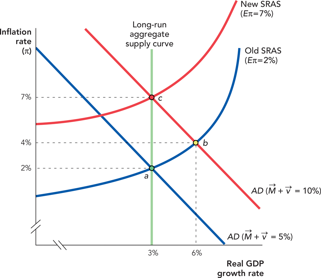
Now that we have covered the major tools of the Federal Reserve, let’s remember that what the Fed ultimately wants to do is to use its tools to influence aggregate demand (AD). Let’s imagine, for example, that the Fed wants to increase aggregate demand and it chooses to do so by buying bonds in an open market operation. The bond purchase increases the monetary base and decreases short-term interest rates. The increase in the base increases deposits and loans through the multiplier process, and the decrease in interest rates stimulates investment (and consumption) borrowing. As a result—if all goes well—AD increases. The increase in AD then influences the economy as discussed in Chapter 32 and is shown in Figure 34.3. Beginning at point a, an increase in shifts the aggregate demand curve outward, moving the economy to point b, where inflation and the real growth rate are higher. In the long run, after transition the economy will move to point c with a higher inflation rate (money neutrality again) but a growth rate given by the fundamentals at the long-run potential level.

We now know that the process is not quite so simple. The Fed can buy bonds and increase the monetary base, but these actions do not increase aggregate demand by any guaranteed amount, since we don’t know exactly how much Ml and M2 will go up in response to the higher monetary base. Nor do we know exactly how much the lower interest rates will stimulate investment spending, especially since the Fed has the most influence over short-term rates, while most investment spending will depend on longer-term rates. In addition, all of these processes take time and the lags from action to response are not fixed but may vary. If the Fed acts to reduce interest rates today, for example, it may take 6 to 18 months before aggregate demand and economic growth begin to respond significantly. In the meantime, economic conditions may change.

330

Thus, to estimate the effect of its actions on aggregate demand, the Fed must try to predict and monitor many variables determining the size and timing of the response to its actions. Some of the things the Fed must try to predict and monitor are:

Will banks lend out all the new reserves or will they lend out only a portion, holding the rest as excess reserves?

How quickly will increases in the monetary base translate into new bank loans and thus larger increases in Ml and M2?

Do businesses want to borrow? How low do short-term interest rates have to go to stimulate more investment borrowing?

If businesses do borrow, will they promptly hire labor and capital, or will they just hold the money as a precaution against bad times?

The Federal Reserve’s power should not be underestimated but increasing or decreasing aggregate demand is not like turning a tap on and off. The Fed has a limited set of tools and it must constantly adapt those tools to new circumstances and conditions. We will be taking up the difficulties and dilemmas of monetary policy in the real world at greater length in the next chapter.