Let’s start with the most straightforward case, namely a negative shock to aggregate demand. Suppose, for example, that the rate of growth of the money supply or falls. Imagine, for example, that entrepreneurs are suddenly more pessimistic about the future state of the economy. Entrepreneurs will wish to borrow less, banks will wish to lend less, and the growth rates of M1 and M2 will fall, causing a fall in aggregate demand.

In terms of our basic AD/AS diagram, the AD curve shifts down and to the left, moving the economy from point a to point b as shown in Figure 35.1. Of course, you’re already familiar with that basic result from Chapter 32 on aggregate supply and aggregate demand. As you can see, the negative shock (if not counteracted by the Fed) means that the growth rate of output will decline. If the monetary contraction is severe enough, the rate of output growth can even turn negative, bringing the economy into a recession, just as we have discussed in Chapter 32 and Chapter 34.

Eventually, the economy will recover from the negative monetary shock. If the reduction in is permanent, for example, wage growth will decline from 10% to 5% and the economy will move to point c. But as we pointed out in Chapter 32, wages are often sticky, especially in the downward direction, so it may take time and considerable unemployment before the economy adjusts to the decline in .

But if the Fed can increase the rate of growth of the money supply, reducing interest rates and encouraging more bank lending and investor borrowing, then the AD curve shifts back up and to the right. Using the policy tools outlined in Chapter 34, the Federal Reserve is able to push the AD curve back to its original position so the economy will transition from point b to a, thereby reducing the severity and length of the recession. In essence, instead of allowing the economy to adjust to a decrease in AD, which may require lower growth and higher unemployment, the Federal Reserve quickly restores AD to its previous level.

343

But Figure 35.1 makes monetary policy look too easy—what could be easier than shifting a curve? Two difficulties make it hard for the Fed to get this right all the time:

Figure 35.2 below portrays the more realistic case for monetary policy in which too little stimulation pushes the economy only to point c where growth is still sluggish. But “too much” monetary stimulation pushes the economy to point d with a higher than desirable inflation rate at 9% (and a growth rate that is high but unsustainable in the long run). Only with the “just right” or Goldilocks amount of stimulation does the economy quickly return to its long-run balanced growth path at point a. We would like it if the Fed hit the just right, or Goldilocks, amount of stimulation every time, but don’t forget: Goldilocks is a fairy tale.

Suppose that the Federal Reserve does overstimulate, pushing the aggregate demand curve to “Too much” in Figure 35.2. What then? Remember from our discussion in Chapter 31 that inflation makes price signals more difficult to interpret, creates arbitrary redistributions of wealth, and makes long-term planning and contracting more difficult, among other problems. Thus, we don’t want inflation to be too high. But, we also know from Chapter 31 and Chapter 32 that bringing down the rate of inflation is costly because prices and wages are not fully flexible in the downward direction. That means economies sometimes get stuck between a rock and a hard place—between continuing a costly rate of inflation or reducing it at the risk of a recession.

344

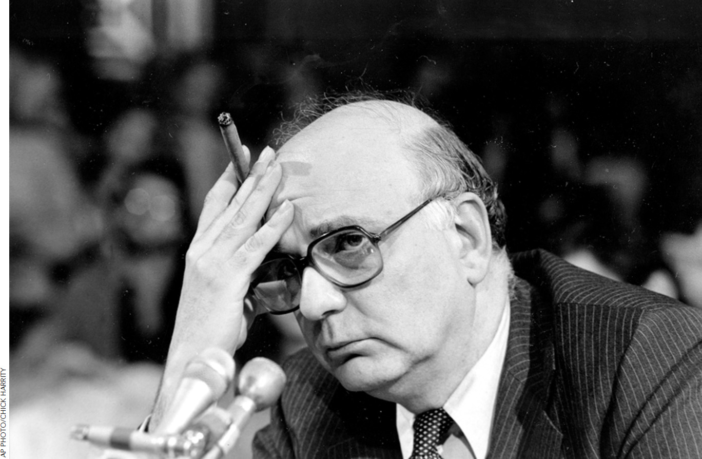
Many economists think that the Federal Reserve did overstimulate the economy in the 1970s; and, as a result, by 1980, the inflation rate hit 13.5% a year. Ronald Reagan was elected to the presidency in part to change economic policies. By 1983, tough monetary policy under Reagan and cigar-chomping Federal Reserve Chairman Paul Volcker had reduced the inflation rate to 3%, but the consequence was a very severe recession with an unemployment rate of just over 10%.

345

The disinflation experiment was costly, but unlike the deflation of the Great Depression, when prices fell, it was a policy chosen on purpose. The 1980s disinflation broke the back of inflation and provided the foundation for the 25 or so years of successful economic growth—and mostly low unemployment—that the American economy enjoyed until the recession of 2008–2009.

Since World War II there have been six episodes when the Fed deliberately put the brakes on money growth, most prominently the shift beginning with the 1980 presidential election just mentioned. In every case, the tighter monetary policies were followed by declines in output. On average, industrial production, 33 months later, was 12% lower than otherwise would have been expected. But again, these contractions aren’t always bad. Sometimes a contraction is necessary to bring down the rate of inflation. Of course, economists debate which of these contractions were needed and which were not.

Whether or not a particular contraction is a good idea, economists do agree on one point: A monetary contraction goes best when it is credible, namely when market participants expect the central bank to carry through its tough stance. This makes sense if you think through exactly why a disinflation is difficult for an economy. A sufficiently radical disinflation leads to unemployment because wages and prices are sticky, especially in the downward direction (as explained in Chapter 32). If nominal wage growth is too high, some workers will end up being very expensive and employers will choose to lay them off. So, the key to a less painful disinflation is to increase nominal wage flexibility. Now imagine that a central bank has announced a disinflation but no one really believes it, or people believe it only halfheartedly. Nominal wages probably aren’t going to grow more slowly, and when the disinflation comes, if indeed it does come, the unemployment cost will be high. Alternatively, if the coming disinflation is widely expected, then workers will be prepared for slower wage growth and will quickly adjust to what they know is inevitable. Thus, a credible disinflation reduces the unemployment effects of disinflation. So, the lesson is this: If a central bank wishes to undertake a disinflation, it has to be ready to stay the course and it should announce and explain its policy very publicly. This is called making monetary policy credibile.

Fear and confidence are some of the most important shifters of aggregate demand. And one of the Federal Reserve’s most powerful tools is not its influence over the money supply but its influence over expectations, namely its ability to boost market confidence. Recall from Chapter 33 that when investors are uncertain, they often prefer to wait, to delay, and to try to gather more information, before they commit themselves. In addition, remember that one reason we see a lot of time bunching or clustering of investments is that it pays to coordinate your economic actions with those of others—that is, you want to be investing, producing, and selling at the same time that others are investing, producing, or selling. Uncertainty, therefore, can create what economists call a bandwagon effect on investment—I am uncertain and so delay my investments, you follow suit not because of uncertainty alone but because your investment is less likely to work well if it doesn’t happen at the same time as my investment (time bunching or coordination of investment). Moreover, the fact that you cut back investment verifies that my decision to cut back was a good idea so no one can be accused of behaving irrationally.

346

Uncertainty drives people away from investment spending and toward assets like cash. Holding cash isn’t very productive but cash and other similar assets are what you want when you are in “wait and see” mode. In terms of our model of aggregate demand, an increase in the demand for cash is indicated by a decrease in . At the same time, increased uncertainty will lead to a fall in , as both borrowers and lenders will cut back, and Ml and M2 will grow at lower rates. Both the and the changes work to shift the aggregate demand curve inward or to the left as in Figure 35.1 near the beginning of this chapter.

To cite an example, uncertainty increased after the terrorist attacks of September 11, 2001. Although the devastation in Manhattan was extreme, the economic cost of the attack was small relative to the size of the U.S. economy. Nevertheless, if enough people had taken the attack as a signal to reduce investment, the bandwagon effect could have created a severe recession. The Federal Reserve stepped in to try to prevent this from happening by lending billions of dollars to banks. In the week before September 11, for example, the Federal Reserve lent about $34 million to banks, a trivial amount. On September 12, the Federal Reserve lent $45.5 billion to banks.

The mere fact that the Federal Reserve sent a countersignal—we are going to massively maintain or increase AD if necessary—helped stabilize expectations, reduce fear, and raise confidence. The Federal Reserve can’t always prevent an increase in uncertainty from reducing and ; sometimes uncertainty really does increase, such as when a war is imminent, and waiting is the appropriate response. But the Fed often can reduce the bandwagon effect and stabilize expectations toward a more positive outcome.

Monetary policy is often about changing expectations and perceptions, rather than just manipulating numbers and equations. That’s one reason why central banking can be so difficult and why it is an art as well as a science.