Let’s use a spreadsheet to compute the elasticity of demand along the two demand curves illustrated in Figure 5.1.

The first step is to input the basic data into the spreadsheet. For demand curve I, we have Q_Before = 100, Q_After = 95, P_Before = $40, and P_After = $50, and for demand curve E, we have Q_Before = 100, Q_After = 20, P_Before = $40, and P_After = $50. (By the way, it doesn’t matter which price–quantity pair you call before and which after.) Your spreadsheet should look like Figure A5.1.

Now remember our formula for calculating an elasticity:

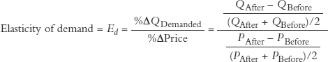
Let’s input the formula in two parts: the %ΔQ on the top and %Δ Price on the bottom, as in Figure A5.2.

94

Notice the formula in cell C2, = (B2 − A2)/((B2 + A2)/2) × 100; that’s the percentage change in quantity along demand curve I. There is a similar formula in C4 for the percentage change in price and then these are repeated for demand curve E.

We can then finish off the spreadsheet by dividing C2/C4 and taking the absolute value, which gives us Figure A5.3.

Fortunately, the answer is consistent with what we said earlier in the chapter! Along this region of demand curve I, the elasticity is 0.231 < 1 or inelastic, and along this region of demand curve E, the elasticity is 6 > 1 or elastic.