Optimization and Consumer Choices
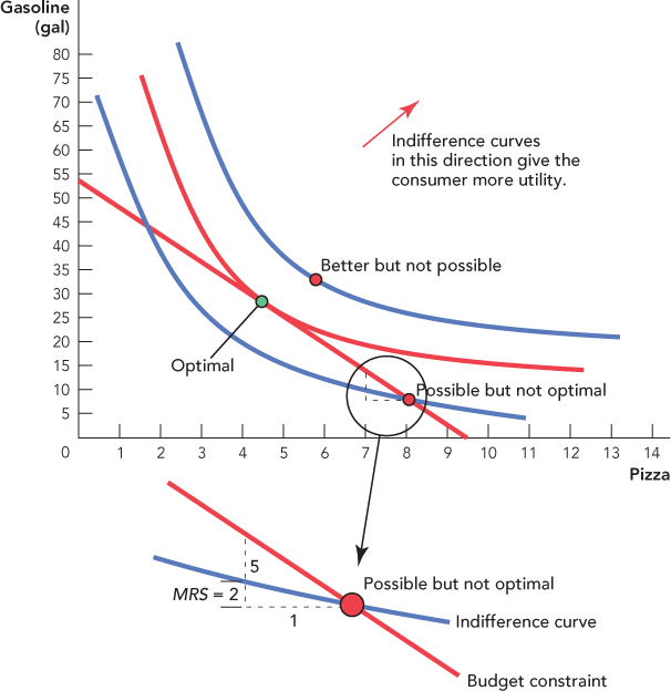
Now that we understand budget constraints and preferences, we can find the consumer’s optimal consumption bundle. We know that the consumer must be on (or inside) the budget constraint and the consumer wants to be on the indifference curve that is the farthest to the northeast. Thus, to find the optimal consumption bundle, we look for the consumption bundle that is on the highest indifference curve but still on the budget constraint. Figure 25.9 illustrates.

 . The “Better but not possible” bundle has more gasoline and more pizza than the bundle labeled “Optimal” but it is not on the budget constraint and thus not affordable.
At the “Possible but not optimal” bundle the MRS = 2 and the slope of the budget constraint,
 = 5. What this means is that the consumer will accept 2 gallons of gas to give up 1 pizza but the market is willing to give the consumer 5 gallons of gas if they give up 1 pizza—that is a good deal! The consumer, therefore, will trade pizza for gas until the MRS =
  .
.474
Notice from Figure 25.9 that at the optimal bundle, the slope of the indifference curve is equal to the slope of the budget constraint. This is not an accident but a requirement. To see why, try to “push” an indifference curve as far as you can toward the northeast while still keeping at least one point on the budget constraint. The point of maximum utility is found where the indifference curve has been pushed so far it just touches the budget constraint.
More formally, consider the point labeled “Possible but not optimal.” This point is on the consumer’s budget constraint, which explains why it is possible. Why isn’t this point optimal? At “Possible but not optimal,” the slope of the indifference curve is 2, which means that the consumer needs just 2 additional gallons of gas to be indifferent to giving up 1 pizza. The slope of the budget constraint is 5, which means that the consumer can get 5 gallons of gas if he gives up 1 pizza—that’s more gas than he requires to be indifferent! Thus at “Possible but not optimal,” the consumer can increase his utility by buying more gas and fewer pizzas and therefore this point cannot be optimal. In fact, what we have just shown is that the consumer can always do better if the slope of the indifference curve is different from the slope of the budget constraint.
Thus, remembering that the slope of the indifference curve is the MRS and the slope of the budget constraint is the price ratio, we can write that the optimal consumption bundle is found where

475
Perhaps you are wondering how  relates to the optimal consumption rule stated earlier:

or rearranging

Can you guess what we are going to say next? Correct, it turns out that  , so fortunately our two conditions for optimal consumption,
  and
and  , are really just two ways of writing the same thing.*
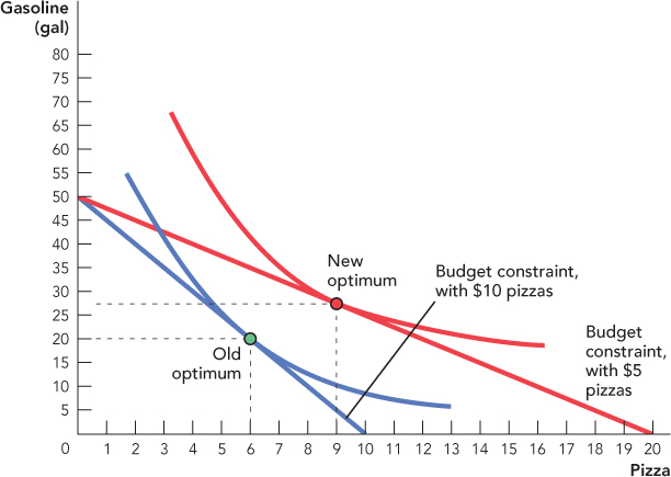
Now that we know how to find the consumer’s optimal consumption bundle, we can show how the optimal bundle changes as income and prices change. Figure 25.10, for example, shows how a consumer responds to a decrease in the price of pizzas from $10 to $5. When PPizza = $10 and PGas = $2, the consumer maximizes utility by choosing 6 pizzas and 20 gallons of gas at the point labeled “Old optimum.” As we showed in Figure 25.6, a decrease in the price of pizzas rotates the budget constraint along the horizontal axis. With the new budget constraint, the consumer chooses 9 pizzas and 27.5 gallons of gas at the point labeled “New optimum.”

476
Notice that a fall in the price of pizza increases the number of pizzas purchased, but in this example it also increases the number of gallons of gasoline consumed. At first, this result may seem confusing: Why should a fall in the price of pizza increase the consumption of gasoline? The reason is that a fall in the price of pizza has two effects, the income effect and the substitution effect. Let’s now explain these two effects.