8.3 OUR GENETIC HISTORY
Genomics research carries important implications that go to the heart of human existence. Where did we come from? How did we get to where we are now? Genomics provides an especially informative and often quantitative window on evolution, ultimately advancing the scientific answer to these and many other fundamental questions. A quest to understand how we came to this point in time is not simply an academic exercise. A better understanding of how new species evolve and how we are related to one another and to other species is highly relevant to advancing knowledge in areas ranging from ecosystems to pandemics. Answers can pay huge dividends in medicine, agriculture, resource management, and general quality of life.
281
All Living Things Have a Common Ancestor
One goal of modern genomics and evolutionary biology is the reconstruction of the evolutionary tree that traces the origin of every extant species. We can approach this problem from both ends—
The successful living entity that gave rise to all life now on Earth is referred to as LUCA, the last universal common ancestor. Although its biological form and genome are obscured by billions of years of evolution, there are several approaches to thinking about LUCA. The first approach, which has been greatly facilitated by modern genome sequencing efforts, attempts to assemble the list of genes and other features that are currently shared by every living organism: these features were probably present in LUCA. The second approach is an effort to define the minimum set of genes necessary to support a living cell. Such a minimalist cell would help define the essence of the free-
As revealed by genomics and work in many other biological fields, current organisms share several features that permit a trace to a common ancestor. The core components of the translation and transcription machinery in all cells are demonstrably related. The use of the d isomers of sugars in cells and the l isomers of amino acids in protein synthesis is also universal. Beyond this point, the generalities start to break down. All organisms consist of cells surrounded by lipid-
Current estimates for the number of genes shared by all known species vary from 80 to about 500. The lower number focuses on genes with clearly identifiable orthologs in all organisms, based on sequence comparisons. The higher number includes genes required for processes that are found in all organisms, but for which many mechanistic and sequence similarities have been obscured by evolutionary time. A cell with 500 components would be simpler than most existing life forms, but still very complex. There must have been many intermediates of gradually increasing complexity in the process that led to LUCA.
The search for the minimal genome begins with the assumption that this cell will grow in a stress-
The bacterium Mycoplasma genitalium, a parasite of the genital and respiratory tracts of primates, has the smallest genome sequenced thus far for a defined organism. Its 580,000 bp DNA includes 521 genes, 482 of which encode proteins. Directed efforts to disrupt individual genes have revealed that the bacterium can dispense with only 97 of them and still retain viability in the laboratory, giving a minimal complement of 385 genes. The small genome of this Mycoplasma reflects its sheltered environment as a parasite.
Similar experiments have indicated that the minimal genome for an organism living autonomously includes about 1,350 genes. Attempts to define a minimal gene complement are fueling efforts to create an artificial cell from nonliving chemical components, an achievement that would mark a new level of understanding of living systems.
Genome Comparisons Provide Clues to Our Evolutionary Past
The evolutionary relationship among species, populations, or genes is known as a phylogeny, and the study of such relationships is called phylogenetics. Phylogenetics helps biologists classify organisms. It can also reveal important information about the evolution of traits in an organism or the appearance of new pathogens. It can even aid in criminal investigations (Highlight 8-2). Phylogenies are usually described with the aid of phylogenetic trees, which can be based on sequence information or on other attributes of a species, such as morphological characteristics. The construction of evolutionary trees was imprecise and descriptive until the 1950s, when mathematical biologists began to systematize the process. That work continues.
HIGHLIGHT 8-2 EVOLUTION: Phylogenetics Solves a Crime
In the summer of 1994, a nurse in Lafayette, Louisiana, broke off a 10-
Investigators found records indicating that the doctor had treated and drawn blood from his only HIV-
Once HIV begins to replicate in a new host, the virus mutates rapidly, an evolution that occurs within one infected individual. Samples taken from a person with HIV years after infection can be used to build a phylogenetic tree that can trace the evolution of the virus in that individual. Blood samples were collected from the doctor’s HIV-
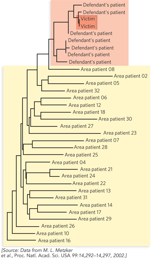
With this and other evidence, the doctor was convicted of attempted second-
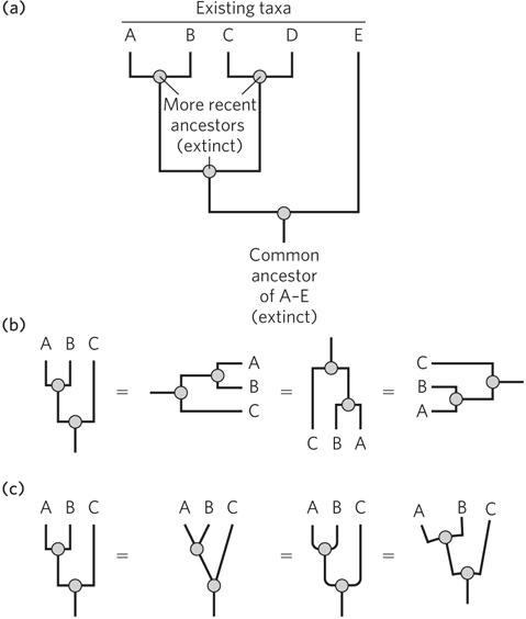
On one level, the branched evolutionary trees often depicted in popular or scientific literature are almost self-
282
283
Branch length can be meaningless, but often it is used to represent some measure of evolutionary time, such as numbers of altered morphological features, numbers of mutations in one or several genes (more common in modern trees), or numbers of genomic alterations in a region of the genome (Figure 8-16a). For example, we can look at the differences in a gene found in both humans and chimpanzees and determine which variant existed in the common ancestor, such as by examining outgroups, as described in Section 8.1. Once the sequence of the gene in the common ancestor is determined, the common ancestor becomes a node in the tree. The lengths of the branches leading from ancestor node to humans and chimpanzees reflect the number of changes occurring between that ancestor and the living species.
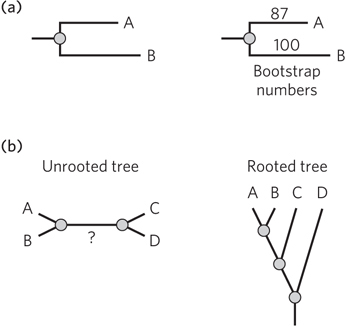
Numbers next to branches on a tree usually reflect the level of confidence the investigator has in the information contained in that branch (see Figure 8-16a, right). A common method for setting confidence limits is the bootstrap analysis, which gives a range from 100 (very high confidence) to 0 (no confidence). In brief, the bootstrap is a statistical method that starts with the set of sequences used to generate the original tree. For example, let’s say a particular sequence of gene X is used to construct a tree for 100 species that all have gene X. A computer program randomly samples the original 100 sequences to create a new set of 100 sequences. In this new set, some of the original set may be missing, and other sequences may be included multiple times. A new phylogenetic tree is generated from each of the created datasets, and the number of times the same branch configuration arises for a cluster of species is tallied. The score reflects the absence (high confidence) or presence (lower confidence) of viable branching alternatives.
An unrooted tree is one for which the positioning of the common ancestor is uncertain (Figure 8-16b). In such a tree, the direction of evolution for parts of the tree might be unknown.
A wide range of problems arise in the construction of evolutionary trees. Mutation rates are often assumed to be constant, but this assumption is flawed. Mutation rates can be affected by environmental factors. For example, reactive oxygen species are the most common source of mutagenic DNA lesions (as described in Chapter 12). Thus, aerobic organisms are subject to more DNA damage and potential mutagenesis than anaerobic organisms. Exposure to DNA-
284
Gene gain can result from a process called horizontal gene transfer, which is common in bacteria and archaea (witness the very rapid spread of genes encoding antibiotic resistance in human bacterial pathogens). Early viruses may have transferred genes from one bacterium to another, and from one species to another, resulting in the sudden appearance (rather than the gradual evolution) of a gene in a particular evolutionary line. Large genome rearrangements might abruptly break up a pattern of synteny in one ancestral line, complicating the analysis. Sorting out these patterns is the job of increasingly sophisticated computer algorithms.
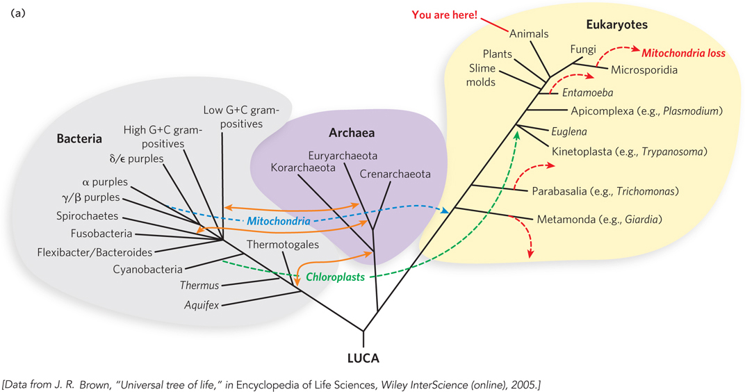
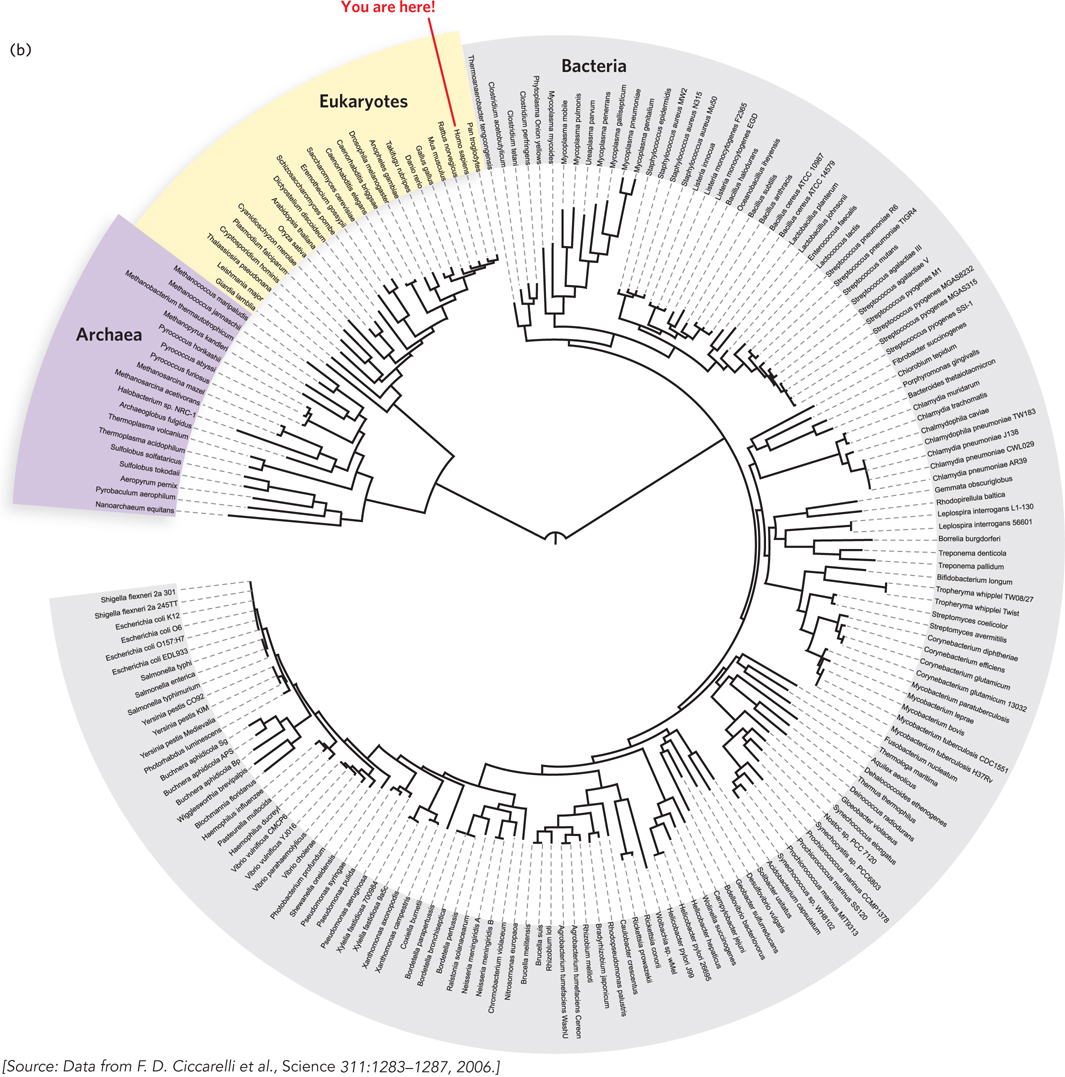
The complexity of the problem is evident in a current tree of life, two versions of which are shown in Figures 8-17a and 8-17b. These trees are based on analyses of particular genes and patterns in fully sequenced genomes. They are probably not correct in every detail. Corrections, additions, and updates will continue for decades, perhaps centuries, to come.
The Human Journey Began in Africa
Four major factors affect the evolution of any group of organisms. Mutation rates determine the extent of genetic diversity. Natural selection affects which genomic changes are inherited in a population. Many mutations are relatively neutral, however, and do not undergo positive or negative selection. Neutral mutations are subject to a third evolutionary factor called genetic drift, in which the frequency of particular mutations in a population changes more or less randomly over time. Genetic drift is affected by such variables as the number of reproducing individuals in a population and the number of offspring generated. Finally, when groups of organisms colonize new regions and environments, their migrations may subject them to new and different selective pressures. All of these forces shaped the evolution of Escherichia coli; they also shaped the evolution of Homo sapiens.
285
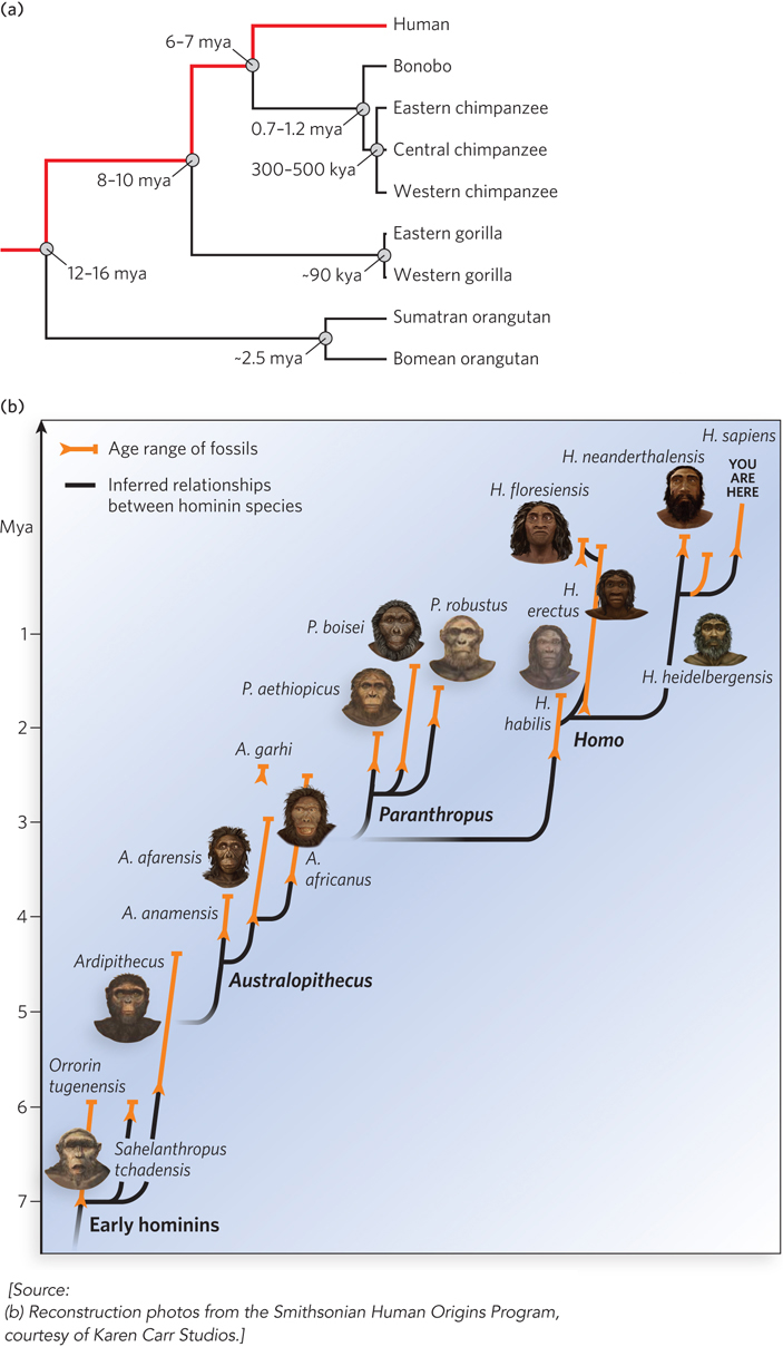
About 7 million years ago, the common ancestor of chimpanzees, bonobos, and humans lived in Africa. Groups of that ancestral species followed divergent lines of evolution, one leading to chimpanzees and bonobos, and one leading to humans (Figure 8-18). The path to humans first generated a series of species in a genus dubbed Australopithecus. The Australopithecines remained in Africa, giving rise, about 3 million years ago, to Homo habilis, the first species of our own genus. The archaeological record indicates that H. habilis was the first species to use stone tools. About 1.7 million years ago, a successor to H. habilis emerged—
286
Homo sapiens evolved about 500,000 years ago. For decades, scientists argued about two possible human origins. The multiregional theory proposed that humans evolved gradually in many places, with gene flow occurring constantly between the various populations. This would entail a direct evolution of H. erectus into H. neanderthalensis into H. sapiens, occurring simultaneously in Eurasia and Africa. The alternative, “out of Africa” theory posits that the H. erectus and H. neanderthalensis expansions into Eurasia were independent of the H. sapiens expansion, and that the former two species represented separate evolutionary branches. Modern genomics has definitively resolved the debate in favor of the “out of Africa” theory.
287
A woman who lived in sub-
There is also a genomic Adam, but Eve never knew him. All males now living on Earth are descended from a male who lived in Africa about 60,000 years ago. Again, Adam was not the only male member of his species present. He is simply the one whose DNA survives. Our information about this individual comes from analyses of haplotypes in Y chromosome DNA, most of which is not subject to recombination.
Human Migrations Are Recorded in Haplotypes
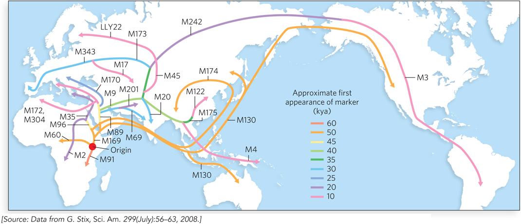
About 50,000 years ago, a small group of humans looked out across the Red Sea to Asia. Perhaps encouraged by some innovation in small boat construction, or driven by conflict or famine, or simply curious, they crossed the water barrier. That initial colonization, involving perhaps 1,000 individuals, began a journey that did not stop until humans reached Tierra del Fuego (at the southern tip of South America) many thousands of years later. In the process, the established populations from previous hominid expansions into Eurasia, including H. neanderthalensis and H. erectus, were displaced. The Neanderthals disappeared, as did H. erectus (Highlight 8-3).
HIGHLIGHT 8-3 EVOLUTION: Getting to Know the Neanderthals
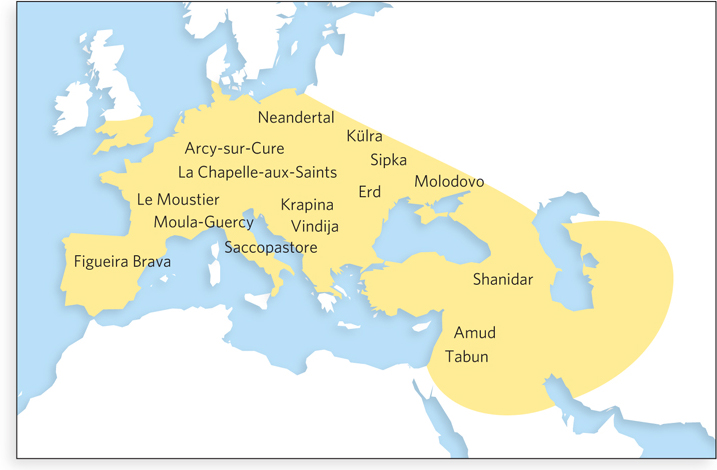
Modern humans and Neanderthals coexisted in Europe and Asia as recently as 30,000 years ago. The human and Neanderthal ancestral populations permanently diverged about 370,000 years ago, but they are the closest known hominid relatives of modern humans. Neanderthals used tools, lived in small groups, and buried their dead. For hundreds of millennia, they inhabited large parts of Europe and western Asia (Figure 1). Buried in the bones and remains taken from burial sites are fragments of Neanderthal genomic DNA. Technologies developed for use in forensic science (see Highlight 7-1) and studies of ancient DNA have been combined to allow the complete sequencing of the Neanderthal genome. If the chimpanzee and bonobo genomes can tell us something about what it is to be human, the Neanderthal genome can tell us more.
This endeavor is unlike the genome projects aimed at extant species. The Neanderthal DNA is present in small amounts and is contaminated with DNA from other animals and bacteria. How does the researcher get at it, and how can we be certain that the sequences really came from Neanderthals? The answers have come from a new application of metagenomics (see Highlight 8-1). In essence, the small quantities of DNA fragments found in a Neanderthal bone or other remains are cloned into a library, and the cloned DNA segments are sequenced at random, contaminants and all. The sequencing results are compared with the existing human genome and chimpanzee genome databases. Segments derived from Neanderthal DNA are readily distinguished from segments derived from bacteria or insects by computerized analysis, because they have sequences closely related to human and chimpanzee DNA. Once a collection of Neanderthal DNA segments is sequenced, they are used as probes to identify sequence fragments in ancient samples that overlap with these known fragments. The potential problem of contamination with the closely related modern human DNA can be controlled for by examining mitochondrial DNA. Human populations have readily identifiable haplotypes (distinctive sets of genomic differences; see Figure 8-7) in their mitochondrial DNA, and analysis of Neanderthal samples has shown that their mitochondrial DNA has its own distinct haplotypes.
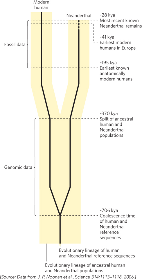
The Neanderthal genome was completed in 2013. The data provide evidence that modern humans and the Neanderthals who were the source of this DNA shared a common ancestor about 700,000 years ago (Figure 2). Analysis of mitochondrial DNA suggests that the two groups continued on the same track, with some gene flow between them, for about 300,000 more years. The lines split for good long before the appearance of anatomically modern humans, although the presence of small bits of Neanderthal DNA in human genomes indicates some relatively late interbreeding. Excluding transposons, the nucleotide sequence of the Neanderthal genome is 99.8% identical to that of the human genome. The sequence comes from a girl whose bones were left in a Siberian cave. We know that her parents were related at the level of half-
Expanded libraries of Neanderthal DNA from different sets of remains should eventually allow an analysis of Neanderthal genetic diversity, and perhaps Neanderthal migrations. This look at the hominid past promises to be fascinating.
This journey can be traced by looking at our genomic polymorphisms. Efforts are under way to survey genetic diversity in human populations around the globe. One such endeavor is the International HapMap (haplotype map) project; another is the Human Genome Diversity Project. Both are international efforts to sequence thousands of human genomes taken from carefully selected populations around the world, and to accumulate information about tens of thousands of polymorphisms in the sequenced genomes. These enterprises are every bit as large and complex as the original Human Genome Project. The results have helped define mitochondrial Eve and Y chromosome Adam, and they are telling us a great deal more. Complementary analyses of mitochondrial DNA from Neanderthals and Denisovans, another hominid group recently discovered in the Denisova Cave in Siberia, have established that they were on a separate evolutionary line.
Phylogenetic analyses of species evolution generally rely on gene mutations that are fixed in a given species: all the members of species X have one gene sequence, and all the members of species Y have a different sequence. The analysis of genetic polymorphisms within a species increasingly relies on a different kind of mathematical analysis, called coalescent theory. Even though it is not subject to recombination, the sequence of mitochondrial DNA, like that of chromosomal DNA, changes slowly with time because of mutations. If a mutation occurred recently, it will appear in the relatively few individuals descended from that female. If the mutation appeared much earlier, it is found in many individuals across broad geographic regions. With mathematical models that take into account estimated mutation rates, selection, genetic drift, and other factors, various polymorphisms are traced back to the ancestor in which they first appeared—
Overall genetic diversity in the human lineage is lower than that in chimpanzees. This is one of several pieces of evidence indicating that early human populations went through evolutionary bottlenecks a few hundred thousand years ago, when only a few thousand or tens of thousands of individuals existed and genetic diversity was limited. Our mitochondrial Eve and Y chromosome Adam lived in times when there were far fewer humans than today. More than 85% of the polymorphisms in the human population appear at the same frequency in all human populations worldwide, indicating that they arose before the appearance of the first modern humans. The remaining 15% tell us about human migrations.
Genetic diversity, in terms of haplotypes that do not occur uniformly across world populations, is by far the greatest in extant African populations. When that wanderlust-
288
Our genomic sequences also tell a story of our interaction with other hominids. During their migrations across the planet, humans encountered Neanderthals and Denisovans. The interactions were clearly complex. Some rare but identifiable interbreeding occurred between humans and these groups, and the evidence remains in our DNA.
289
Of course, similar methods can be used to analyze the history of any species, from viruses to mammals. For example, these methods allow the tracing of viral evolution associated with human pandemics and reveal the types of mutational events that occurred in the past and are therefore possible in the future. Related methods are used to predict which influenza virus variants will be prevalent in the coming flu season, and thus guide the production of vaccines. Analysis of the genomic history of maize or rice could reveal lost genetic diversity in common production strains that might prove useful to agriculture.
The ongoing analysis of worldwide human genetic diversity—
290
SECTION 8.3 SUMMARY
Genome studies have facilitated new approaches to defining the last universal common ancestor, LUCA. Genomics is used to identify genes that are common to all extant life forms and were therefore likely to exist in LUCA.
Perhaps the ultimate challenge of genomics is to define the tree of life, a detailed description of the evolutionary history and relationships of all species now living on Earth. An evolutionary tree is referred to as a phylogeny; phylogenetics is the study of evolutionary relationships.
The study of mitochondrial DNA, Y chromosome DNA, and genetic haplotypes in the human population enables geneticists to trace human evolution and more recent human migrations.
UNANSWERED QUESTIONS
Genomics, transcriptomics, and proteomics are disciplines designed to obtain large amounts of information about an organism and the systems within it. The list of accomplishments is long, but the list of questions is even longer. There is a rich but largely unpredictable future in these fields.
How many classes of RNAs exist in cells, and how do we find the corresponding genes? The discovery of new classes of RNA is a rapidly evolving area of research. Among these are RNAs involved in all kinds of processes, most notably regulation. Some of this research is described in Chapter 22.
Are there additional domains of living organisms? The 1977 discovery of the archaea surprised many researchers. These microorganisms are now firmly established as a distinct branch of the evolutionary tree, separate from the eukaryotes and bacteria. Is there another domain we have missed, or even more than one? There are certainly sufficient numbers of unusual life-
sustaining niches on Earth to make this plausible. What are the most likely characteristics of LUCA? Ongoing endeavors to define the complete tree of life will gradually refine our understanding of how biological evolution proceeded. Aided by new sequence information, increased knowledge of mutagenesis and nonlinear events that contribute to evolution (horizontal gene transfer and transposon introduction), and complementary data from other fields (including more precise dating methods), we can expect an ever more detailed tree of life in the decades ahead. A parallel effort to better define the processes common to living systems and those that must have been present in LUCA may provide us with a look at our deepest biological past.
How do we investigate interdependent microbial communities? The new field of metagenomics is starting to tackle questions about the diversity of unculturable bacterial species in environments such as the digestive tract of termites. New approaches will be needed to generate complete genome sequences of the many members of such communities and to analyze the genomes for clues about why individual species cannot survive without the others present. The human microbiome, with all of its implications for human health, is an especially important challenge.
291
What evolutionary innovations define humans as a species? Among the many subtle differences we can see between the human genome and other primate genomes are mutations of many kinds that hold the key to our capacity for higher thought, language development, and other human traits. Understanding these will advance our understanding of medicine and neurochemistry in myriad ways, some of which we cannot predict.
Personal genomes are in our future, but how will they be used? The science of extracting information from our genomes is still in its infancy. We don’t yet understand the function of many of our own genes. The impact of personal genomes on medicine will increase as that understanding grows.
292
Haemophilus influenzae Ushers in the Era of Genome Sequences
Fleischmann, R.D., M.D. Adams, O. White, R.A. Clayton, E.F. Kirkness, A.R. Kerlavage, C.J. Bult, J.F. Tomb, B.A. Dougherty, J.M. Merrick, et al. 1995. Whole-
The first genome sequencing projects, in the early 1990s, used this strategy: clone, map carefully, and then sequence. Craig Venter, who had recently established The Institute for Genome Research (TIGR), was eager to test his idea that, by using new computational methods, one could skip the time-
H. influenzae was first described by Richard Pfeiffer in 1892 during an influenza outbreak. Until 1933, this bacterium was incorrectly thought to be the cause of the common flu. There are six types of H. influenzae (designated a through f) that can be immunologically distinguished by differences in their polysaccharide coat or capsule, and many other unencapsulated types. This bacterium is an opportunistic human pathogen that lives in tissues and rarely causes disease. However, H. influenzae type b is responsible for acute bacterial meningitis and bacteremia, primarily in children.
The organism chosen for analysis was Haemophilus influenzae Rd, a well-
The DNA isolated from H. influenzae was sheared mechanically and size-
Next, the computer algorithm tackled the immense job of assembling the genome by building a table of all 10 bp oligonucleotide subsequences and using the table to generate a list of potential fragment overlaps. With a single DNA fragment beginning the assembly of a contig, candidate overlap fragments were chosen and tested for more extended matches by strict criteria. Gradually, overlapping fragments were pieced together to generate a genome sequence. Assembling the 24,304 fragments required 30 hours of computer time. When the assembly was complete, the fragments had been ordered into 42 contigs, with 42 gaps in the genome and little information about how to order the contigs. However, many of the gaps were short. Sometimes a contig end fell within the same single gene as another contig end, both being identified by virtue of existing peptide sequences for the gene in question. Additional libraries containing long clones of H. influenzae DNA were probed with sequences near contig ends, to identify ends that were near each other. The gaps were closed by this method and by other targeted sequencing efforts.
By the end, the genomic sequences of the bacterium had been sequenced with more than sixfold redundancy. The final error rate was estimated at 1 in 5,000 to 10,000 bp. At $0.48 per finished base pair, the total cost was just under $900,000. Newer sequencing technologies, such as those described in Section 7.2, have lowered the cost of sequencing a typical bacterial genome by almost three orders of magnitude.
The result of Venter and colleagues’ endeavor was a complete genome sequence with 1,830,137 bp, published in July 1995. The genome included 736 predicted genes, over half of which had no known function at that time. More importantly, the effort inspired a new generation of genome analysts. TIGR is now the J. Craig Venter Institute, and it remains a major force in genome sequencing. The shotgun sequencing approach successfully pioneered in the H. influenzae study is now routinely paired with the new sequencing technologies to provide rapid and inexpensive genome assemblies.
293