Chapter 1. Introducing Statistics
Introduction
Are you curious about the world around you? Are you interested in ways to describe patterns and trends? Would you like to draw conclusions—or evaluate the conclusions of others—based on the evidence you see? If you answered "yes" to any of these questions, then statistics can be a valuable tool for you.
Whether you are studying statistics because it sounds interesting or because it is required for your educational program, you will be able to find many applications that interest you. Statistical techniques are used in a broad range of fields, including sports management, computer engineering, sustainable agriculture, supply chain management, social work, and criminal justice. Both professional journals and popular media present results of statistical analysis; whatever your field of study, you are likely to encounter statistics along the way.
1.1 What is Statistics?
Statistics is the process of collecting, describing and drawing conclusions about data. But what, you may ask, are data? Data are measurements or observations made about the people or objects we are investigating.
In this section we look briefly at the process of statistics, considering examples that illustrate the ideas we will study throughout the course. In each case, we will consider several questions.
What is the question of interest? Before we begin to use statistics, we should identify exactly what we are interested in finding out. Do we want to investigate a relationship between two or more characteristics? Are we trying to gauge public opinion or behavior on a certain topic? Do we want to summarize the results of some event or activity? Are we trying to verify the safety of a product or the effectiveness of some treatment? All of these are appropriate reasons to use statistical techniques. As we shall see throughout this course, determining exactly what technique to use depends in large part on our question of interest.
From what individuals were data collected? When we use the word “individuals” in everyday English, we are generally referring to people. In statistics, individuals are whatever we want to learn about—whether people, animals, or inanimate objects. Each datum (the singular of the word data) is a little piece of information about an individual. When a set of data is collected, we have one or more pieces of information about each individual.
What measurements or observations were made? The measurements or observations made are, in fact, the data collected. What we measure or observe can be something we count (like the number of siblings a person has), something we measure (like the miles per gallon for a certain model of car), or something non-numerical (like the color of a bird). Sometimes we are interested in only one piece of information for each individual; sometimes we are interested in two or more.
How were the data presented? Raw data consists of lists or tables of the observations. Unless we are collecting a very small set of data, raw data is difficult to use. Thus, we frequently summarize the data, either using a graphical, verbal, or numerical description to explain any patterns or trends.
What conclusions were reported? Our original question of interest tells us why we collected the data. Once we have looked at the data through the “eyes” of statistics, we can report what we learned. Were we able to answer the question, or does it need further study? How sure are we that our results are reliable? Once again, our question guides us in proceeding. If we want to determine whether a certain medication is safe for infants, we want to be much more confident in our results than if we want to know whether the majority of people prefer chocolate ice cream to vanilla.
These are questions that we will be returning to throughout our study of statistics. As you learn more about statistics, you will (hopefully) begin to appreciate the subtleties involved in making decisions using statistics.
1.1.1 Today's College Students' Self Esteem
Much has been made of the supposed off-the-chart self-esteem of today’s young people (encouraged by parents who convinced them of their “specialness”). But, in fact, are current college students more self-centered than in the past?
In February 2007 several major news sources reported the results of a comprehensive study performed by researchers at several major research universities. The participants were 16,475 college students nationwide who completed an evaluation called the Narcissistic Personal Inventory (NPI) between 1982 and 2006. Sample questions from the survey included: “If I ruled the world, it would be a better place,” “I can live my life any way that I want to,” and “I like to be the center of attention.”
The researchers reported that there has been a steady increase in the NPI scores between 1982 and 2006, and that 67% of students had above average scores in 2006 compared to 30% in 1982. The study also suggested that narcissists are “more likely to have romantic relationships that are short-lived, at risk for infidelity, lack emotional warmth, and to exhibit game-playing, dishonesty, and over-controlling and violent behaviors.” The researchers noted that “current technology fuels the increase in narcissism” and “by its very name, MySpace encourages attention-seeking, as does YouTube.”
What is the question of interest? The researchers are interested in whether college students exhibit more narcissistic tendencies today compared to students in the 1980’s.
From what individuals were data collected? In this study, data were collected from 16,475 United States college students between 1982 and 2006.
What measurements or observations were made? For each individual, scores on the Narcissistic Personal Inventory were recorded.
What conclusions were reported? The researchers found that Generation Y students are more narcissistic now than students in the past, and that the percentage of students who have above average scores on the NPI more than doubled between 1982 and 2006.
Such a study may be of considerable interest to you as a current college student, and to your professors as they select educational strategies for their courses. Future employers may wonder how such a psychological profile will impact their workplace policies.
1.1.2 Migraine Treatment
According to the Migraine Research Foundation, over 10% of the population suffers from migraine headaches, with three times as many adult women affected as adult men. If you are a migraine sufferer, you are in good (if painful) company. It is reported that Elvis Presley, Vincent Van Gogh, Elizabeth Taylor, and both Ulysses S. Grant and Robert E. Lee suffered from migraines, as do Whoopi Goldberg and Marcia Cross. For famous and “regular” folks alike, a critical concern is how to best treat a migraine headache.
In a study reported in the Journal of the American Medical Association, a large group of migraine sufferers were divided into four groups to determine the effectiveness of various treatments for their pain. One group was given two drugs, sumatriptan and naproxen sodium, the second group was given sumatriptan only, the third group received only naproxen sodium, and the final group received a placebo, a pill containing no medicine. In the United States naproxen sodium is an over the counter drug (and is sold using the name “Aleve”) whereas sumatriptan is available only by medical prescription.
After two hours, the individuals’ pain was evaluated. The study found that, “The incidence of sustained ( 24 hours) pain-free response was significantly higher with combined therapy (25%) than with sumatriptan (16%), naproxen (10%), or placebo (8%).”
What is the researchers’ question of interest? The researchers are interested in determining whether the use of two medications significantly reduces pain in migraine sufferers; they are attempting to evaluate the relative effectiveness of several different headache treatments.
From what individuals were data collected? The researchers studied many patients (about 3000) with a history of migraine headaches.
What measurements or observations were made? For each individual, researchers recorded which treatment was given, and whether pain was reduced.
How were the data presented? The study reported the percentage of patients experiencing pain relief from each treatment, as well as the likelihood that such results would occur if the treatments were all equally effective. This procedure for comparing results is a commonly used one, and one we will study in more detail later on.
What conclusions were reported? Researchers reported that the two-drug treatment was the best in reducing headache pain.
Question 1.1
A study published in the June 2008 edition of the journal Pediatrics looked at whether parents of overweight teens who correctly recognized their child's weight status engaged in behaviors that helped their child's long-term weight management. The study involved overweight teens in the Minneapolis/St. Paul area who participated in Project EAT (Eating Among Teens) in 1999 and 2004.
Parents were asked, in part, to best describe their child’s current weight and to answer questions such as “Duringthe past week, how many times did all or most of your familyliving in your house eat a meal together?" and “How often are fruits and vegetables available in your house?” The researchers found that parents who acknowledged that their children were overweight were much more likely to encourage their children to diet, but not more likely to offer healthy food choices and better meal practices.
hVQHfF9SbEohpBY643JDlzajHUEQlYuy4OptaaSGRVOhag8U5JzPHAwgZMQu+BtMnJeL4O74EedVeSpdMla2xm1VXXmovzgQSw3LNuaSWF6uax808os+wiTFAOcrjTEO+tCmsq+vvB545wlrU+A/rIkmtqhGYBBEu2I4iT4WpEURJDCjLrl9IcBVX5IRJBrqLbE7LhimCE5cUpzifYVzqooZdhtAJCyPmbTHLOIcXF/CDNwUer0BTw==(b) The individuals were parents of overweight teens who participated in Project EAT.
(c) The observations made were (1) the parents' weight classification of their child, (2) how often fruits and vegetables were available in their house, and (3) the number of times that most of the family living in the house eat a meal together.
(d) The study found that while parents who realized that their children were overweight were more likely to suggest that their children diet, they were not more likely to encourage healthy eating styles.
1.1.3 Election Controversy
While it is now “ancient history,” many die-hard Democrats continue to believe that Al Gore really won the 2000 presidential election. The results of the election came down to the question of who won the state of Florida, George W. Bush or Al Gore. There were many lawsuits filed by both sides, and the outcome was decided in the Supreme Court of the United States in favor of Mr. Bush.
In a particular lawsuit, three Florida voters alleged that the layout of the “butterfly ballot” used in Palm Beach County was in violation of Florida statutes and caused many voters, particularly senior citizens, to “overvote” (vote for more than one candidate) or vote for Pat Buchanan when they intended to vote for Al Gore (“misvote”). Analysis of these results was of interest to statisticians as well; the journal Statistical Science devoted its November 2002 issue to electoral statistics, and included an article about the 2000 presidential election in Florida.
What is the question of interest? The plaintiffs in this lawsuit wanted to show that people who meant to vote for Gore actually voted for Buchanan instead or both Gore and Buchanan; they asked the court to authorize a re-vote in Palm Beach County. They wanted to summarize the results of the election and to explore the relationship between votes for Gore and votes for Buchanan.
From what individuals were data collected? In this instance, the individuals are all counties in Florida.
What measurements or observations were made? For each county, the total number of votes for each candidate was recorded.
How were the data presented? While the lawsuit itself does not include the data, the data and various statistical analyses were a necessary component of the legal argument. Figure 1.1 shows the certified vote totals for all Florida counties.
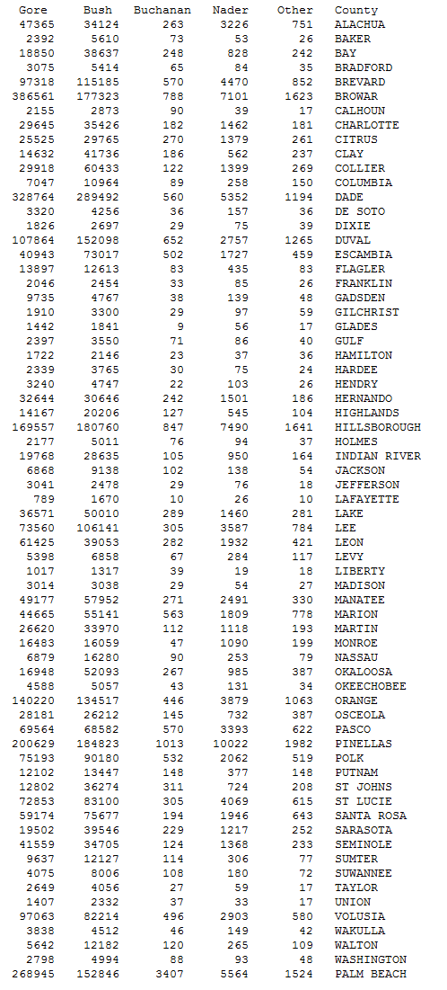
What can we conclude from looking at the numbers in Figure 1.1? Probably not much. Here we see how difficult it can be to work with raw data. Whatever patterns may exist in the data are hard to determine when looking at columns of numbers. What did the plaintiffs (and many other Democrats) see in all of these numbers that led them to conclude that people mistakenly voted for Pat Buchanan in Palm Beach County?
The 2000 presidential election is not unique in generating statistical controversy. In 1936, the Literary Digest incorrectly forecasted that Alf Landon would defeat Franklin Roosevelt. A famous photograph from 1948 shows Harry Truman holding a newspaper whose headline mistakenly predicted his loss to Thomas Dewey. In the next chapter, you can look more closely at the statistical issues involved in these errors.
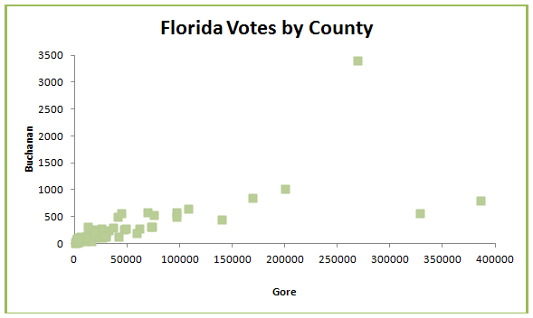
When statisticians compare the Palm Beach results to results in other Florida counties, several discrepancies stand out. One of these is the relationship between the votes for Gore and the votes for Buchanan. Figure 1.2 shows votes for Gore on the horizontal axis and votes for Buchanan on the vertical axis. Do you see an overall pattern? Do you see the point that doesn’t seem to “fit?” That point, showing 268,945 votes for Gore and 3,407 for Buchanan, represents Palm Beach County, historically one of the most Democratic counties in the nation. You would expect that the relationship between votes for Gore and votes for Buchanan to be somewhat consistent. The fact that the Palm Beach County results “stand out” from the rest suggests (at least to the Gore supporters) that something strange happened there.
What conclusions were reported? The plaintiffs in the lawsuit (along with a number of statisticians) concluded that the butterfly ballot caused voting errors, and requested a re-vote in Palm Beach County.
In the end, the U.S. Supreme Court reversed the manual recount ordered by the Florida Supreme Court, and George W. Bush won the 2000 election. He won the 2004 presidential election by a wide margin, avoiding lawsuits and statistical controversies.
1.1.4 Green Living
While Al Gore never became president, he did win an Oscar and the Nobel Prize for his work on climate change. Has increased attention to the environment caused people to make lifestyle changes to live “green”?
In March 2008 a Gallup poll found that 28% of Americans reported changing their shopping and living habits to help protect the environment. The results were based on telephone interviews with 1,012 national adults, aged 18 and older, conducted March 6-9, 2008.
What is the question of interest? The researchers were interested in determining whether Americans have changed their shopping and living habits to help the environment. They were attempting to gauge public behavior.
From what individuals were data collected? In this poll, data were collected from 1,012 U.S. adults, 18 years of age or older.
What measurements or observations were made? For each individual, researchers recorded what kind of changes (major, minor, or no) he or she has made in the past 5 years to help the environment.
How were the data presented? The Gallup Poll reported the percentages of individuals making each level of changes, using a bar graph (Figure 1.3) with actual percentages given.
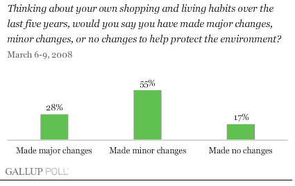
What conclusions were reported? The Gallup organization concluded that “Even though there has been an increased focus on global warming and a growing market of environmentally friendly products, Gallup's annual Environment poll finds just 28% of Americans reporting they have made ‘major changes’ in their lifestyles to protect the environment.” The article summarizes results from various demographic groups, and reports on percentages making particular changes, such as recycling. Notice that along with reporting the results, the Gallup Poll article interprets the results, and discusses the survey methods.
To investigate the variety of careers that employ statistical methods, view the Snapshots: Introduction to Statistics.
The examples presented in this section involve various statistical techniques, and give a preview of some of the topics that we will study in this course. As you watch TV, browse the Internet, or read your favorite magazine, be on the lookout for graphs and discussions that present statistical results. You may be surprised at how often you encounter them!
The questions we asked
- What is the question of interest?
- From what individuals were data collected?
- What measurements or observations were made?
- How were the data presented?
- What conclusions were reported?
are a good starting point for determining how reliable or useful the results may be.
1.2 Data from Populations and Samples
In Section 1.1, we looked at examples that used statistics in different ways and for different purposes. Let’s begin here by contrasting two of these examples.
In the 2000 Florida presidential election example, the purpose was to draw a conclusion about what actually happened. We considered (and compared) the results from every single county in Florida. All of the possible data was available to us. In the final example, about living “green,” the Gallup Poll reported on a survey of 1,012 “national adults,” and concluded that just 28% of Americans reported that they have made ‘major changes’ in their lifestyles to protect the environment.” In this case, all the possible data was not available; the Gallup organization contacted only 1,012 Americans. But the conclusion they want to draw is not just about those people, but about Americans in general.
Here we see an important distinction between two groups of individuals. The population is the set of all individuals that we want to describe or draw a conclusion about. Many times it is either not practical or not possible to collect data from the entire population. (It is not practical to survey all Americans; it is not possible to test a drug on all the individuals who might one day need it.) In such cases, we collect data from a subset of the population; we call this subset the sample. In the previous example, the population is all American adults and the sample is the 1,012 American adults surveyed.
When we collect data from a population or a sample, we are observing or measuring one or more characteristics of the individuals. We call these characteristics variables, because they vary from individual to individual.
The video StatClips: Types of Variables provides an excellent discussion of the difference between quantitative and categorical variables.
Some variables are quantitative; they are numerical in nature, and represent characteristics that we can count or measure. For college students, the number of courses completed and GPA are both quantitative variables. We count the number of courses completed (the value must be a whole number); we measure the GPA (if a 4-point scale is used, the value can be any number between 0 and 4). If we measure a variable, then we usually attach a unit of measure to the result. In the case of GPA (Grade Point Average), the “average” is measured in “points,” typically on a 4-point scale.
Other variables are categorical (or sometimes called qualitative); these are non-numerical characteristics of an individual that are generally described with words rather than numbers. For a college student, place of residence would be a categorical variable, with the values of that variable being on-campus or off-campus housing.
1.2.1 Who?, What?, and Why?
Flip-flops are a common footwear choice among college students when weather permits. While they are cool and comfortable, do they cause problems for students later on? Researchers at Auburn University noticed that students returning from summer vacation often complained about leg and foot pain, and these students seemed more likely to be flip-flop wearers. They wondered whether there was a connection between wearing flip-flips and having foot pain so they undertook a study, using 39 college-aged men and women. They had the volunteers walk on a platform wearing both flip-flops and standard athletic shoes; they measured the vertical force with which the participants’ heels hit the ground, their stride lengths, and their ankle angles. They found that when walking in flip-flops, the individuals’ heels hit the ground with less force, and they had a shorter stride length but a larger ankle angle. This study generates some “who?,” ” what?,” and “why?” questions, which are merely different (easy to remember?) versions of what interested us in section 1.1.
Who? What individuals do the data describe? How many individuals are there? The data describe 39 college-age men and women; this group forms the sample.
What? What variables were observed or measured? Were the variables quantitative or categorical? According to the article, students were observed wearing both flip-flops and standard athletic shoes, and vertical force, stride length and ankle angle were measured. The type of footwear worn is a categorical variable; vertical force, stride length and ankle angle are all quantitative variables.
Why? What was the question of interest in this study? Do these data answer that question? Do we want to draw conclusions about a larger set of individuals? The researchers were interested in determining whether there is a connection between wearing flip-flops and having leg and foot pain. The population would be all people who wear flip-flops since presumably the researchers want to know about all such people (not just college-aged ones). It is not clear from the study whether this connection really exists. What was shown was that wearing flip-flops alters a person’s gait. This alteration in gait may cause foot and leg pain.
Many factors influence a person’s choice of political affiliation. Much has been made of the “gender gap” in politics, but other factors may also influence political party selection. A February 2008 Gallup Poll explored the relationship between marital status and political party preference. A telephone interview was conducted with 12,181 adult Americans who reported their gender, their marital status, and which political party they preferred.
Who? What individuals do the data describe? How many individuals are there? The data describe 12,181 adult Americans and this group of individuals forms the sample.
What? What variables were observed or measured? Were the variables quantitative or categorical? The poll recorded each individual’s gender, marital status, and party identification. These are all categorical variables.
Why? What was the question of interest in this study? Do these data answer that question? Do we want to draw conclusions about a larger set of individuals? The Gallup organization wanted to determine whether there was a relationship between marital status and political affiliation. These data seem to suggest that the two variables are related. The data are used to draw a conclusion about all Americans (the population) based on information from the individuals studied (the sample).
Now let’s look at how the Gallup organization reported the results. They certainly did not report the raw data; rather they summarized what they learned. For example, for unmarried women, 46% of those surveyed considered themselves Democratic, 35% considered themselves Independent/Other, and 17% considered themselves Republican. We call each of these numbers a statistic,because it describes a sample. When we have a number that describes a population (the average length of service of all U.S. senators, for example), we call that number a parameter.
It is sometimes a bit tricky to decide whether you have a statistic or a parameter; the issue is whether the number you are considering describes a sample (then it’s a statistic) or a population (then it’s a parameter). If you calculate the average GPA of your English composition class to verify that your class is an unusually bright group of students, you are finding a parameter. If you are using the average GPA of your English composition class to estimate the average GPA of all English composition students at your college, then you are finding a statistic. Same number, different purposes—it depends on the set of individuals you are trying to describe. In the first case, the population is the students in your English composition class; in the second, the population is all English composition students at your college, and your particular class is serving as a sample.
Notice that we now have the two different meanings of the word “statistics.” In the previous section we defined statistics as the process of collecting, describing and drawing conclusions about data. You might want to think of this as the “big S” definition—the “big picture” description of an area of study. (This use of the word is always plural.) Our new definition of statistics as numbers that describe a sample is then a “little s” definition. We talk about a statistic (singular) if we refer to a single number; we talk about statistics (plural) if we refer to two or more such numbers.
1.2.2 Adding a How?
Open Source Shakespeare is a database containing a wealth of information about the works of William Shakespeare. We can use the website to investigate whether Shakespeare’s tragedies are more complex than his comedies by considering the number of lines, the number of scenes, and the number of characters in each play. For the tragedies, the average number of lines was 1074, the average number of scenes was 24, and the average number of characters was 40. For the comedies, the average number of lines was 906, the average number of scenes was 16, and the average number of characters was 24. In each case, the average for the tragedies is significantly larger than that for the comedies.
We will now add a new question to our list. “How?” will address the manner in which the data are described; in particular, do numerical summaries refer to the entire population or only to a sample?
Who? What individuals do the data describe? How many individuals are there? The data describe 11 tragedies and 14 comedies written by William Shakespeare.
What? What variables were observed or measured? Were the variables quantitative or categorical? For each play, the type of play, the number of lines, the number of scenes, and the number of characters was recorded. The type of play is categorical; each of the other variables is quantitative.
Why? What was the question of interest in this study? Do these data answer that question? Do we want to draw conclusions about a larger set of individuals? The question of interest was whether Shakespeare’s tragedies are more complex than his comedies. Based on the data collected, it would seem that this is the case. The conclusion is only about the plays of Shakespeare, not about a larger set.
How? What numerical summaries were given? Were the numbers parameters or statistics? The average value of each variable (number of lines, scenes, and number of characters) for the two genres was reported. These numbers are parameters because they summarize the variables for all of the tragedies and all of the comedies.
When populations are small, as in the case with Shakespeare’s tragedies and comedies, finding parameters is usually easy enough. But when populations are large, or it is not possible to study all individuals, samples can provide some information that may help us understand the underlying population.
For a number of years doctors have encouraged women to limit their consumption of alcohol and caffeine during pregnancy. Some studies have shown a link between a mother’s high caffeine intake and her baby’s low birth weight. A group of Danish researchers conducted an experiment to investigate the effect of caffeine reduction on both birth weight and length of gestation.
Pregnant women were randomized into either a caffeinated coffee group (568 women) or a decaffeinated coffee group (629 women). Once the babies were born, birth weights and lengths of gestation for 1153 single births were analyzed. The average birth weight for babies born to women in the caffeinated coffee group was 3539 grams; the average birth weight for babies born to women in the decaffeinated group was 3519 grams. The average length of gestation for babies born to women in the caffeinated coffee group was 280.2 days; the average length of gestation for babies born to women in the decaffeinated group was 279.3 days. The differences in average birth weight and average length of gestation were not significant; researchers concluded that “Providing decaffeinated coffee to women who drank three cups of coffee or more a day in early pregnancy had no effect on birth weight or length of gestation.”
Who? What individuals do the data describe? How many individuals are there? The data describe 1153 women who had singleton babies.
What? What variables were observed or measured? Were the variables quantitative or categorical? The researchers recorded whether each mother’s was assigned to the decaffeinated or the caffeinated group and her baby’s weight and length of gestation. The group to which mothers were assigned is a categorical variable; the baby’s birth weight and length of gestation are quantitative variables. Birth weight was measured in grams; length of gestation was measured in days. (If you read the journal article, you noticed that the researchers recorded additional variables, which they used for secondary analysis.)
Why? What was the question of interest in this study? Do these data answer that question? Do we want to draw conclusions about a larger set of individuals? The researchers were interested in determining whether there is a connection between high caffeine intake and low birth weight or shorter gestation. These results suggest that the high caffeine intake is not related to low birth rate or shorter gestation. The researchers want to draw a conclusion about all pregnant women (the population) based on information from the individuals studied (the sample).
How? What numerical summaries were given? Were the numbers parameters or statistics? Average birth weight and average length of gestation were given for the caffeinated and decaffeinated groups. These numbers are statistics because they summarize sample data.
Question 1.2
The accompanying spreadsheet gives water condition data for Huntington Beach, located on Lake Erie in Bay Village, Ohio, for the 2007 recreational season (Memorial Day to Labor Day). These data come from water observations made each morning; the number of E coli bacteria present is used to determine whether it is safe to swim at the beach. (More information about water quality at Lake Erie beaches is available at http://www.ohionowcast.info/index.asp.)
Use the data set to answer each question.
mgW9mKX6IByG3lZOC6i4ib87oOItp5f14iGXIMiDzMT+qF2jhI1efIp3Bhqh1aj8BV7GMgfq7+aJnR1BMM/lTLYrIvOvivdgrwY26M2tzxrafmVQKaOuGHYQCdu2nqQbTV+D+xtmd3iSWNhbw7NYY01XtzU5TDUSv5dtgnf95LAri/7EBcVt8LYlqCbulO1JiUGOnWVBAsQ0JpTuYIdLcgV7uUjIK/WnbaOsZO1Za/cnPkX5qYaUPUEDDecL99hOOznrD4mdycE+qBXdAuFqbpwCCu19rYnQ2mJ4qSOpHWmFkKZiA2+mpMVS3e1Wteh/oIBNi+IFoMD4wY2w30uYl9dqzeopSkcFxr4ztHlMOlbpeDtMqh24wlGfMeKl10Z52WdoTmUZwdNS6hi0xSRVnTcHBOt+vOKkjPzkx5qJ61qfTwAbCYzV3tDLJMn1T6yAOQqDxmTbFaGqvjs9zkkbBZPcVcUmcfN3ZwOLYPI7uBXlrkngTb2Es0XkSmEl4wXLEp0x5IDI/INkf4kwmb5t11SsAk9TmURr19FuVrxhVP7cvgWcuBJrmhbFqu36Z+G46jwZ52z+mPjV4yOFp8dPzz13rOq+/zr7zyP8PPNusjZpvqogxsjahAcBpH9EF8w6D8YO+cNUcv3CDL93la+o9q4Wh9dENTRjew7jctOYCG/vMvSDgqbRZdeUUfRbz/x9UbvvEomFhSPnocM71MeQSZC3+lIl6pL9E5lpmomE+IfB8XmVwS8LBN1Y0ajUS6+dEe6LPo57h6Vh8Z66eDXubXywGg7Xzk8tkuBgpYmZfmxMeBcyirXAQgEEkVCErItGCbl/caIN+InIp+HG9xg2YcvxjoRgB3+Ynk9XyczR+/tHHPRBPwn1daK0GgCyX7yY6NTczlBiV/XNcrfXxA78isdzfaRWcL3JbFYh2qR7f9xgwBucRdK8bvKvkrejeA/xty7actTc3U8PedJzU5//qoI/IRmyfEyOrriz6YQq0LY=(2) The quantitative variables measured were E. coli bacteria, water temperature, and rain in past 48 hours. The categorical variables measured were wave category, water quality, and whether a swimming advisory was in effect.
(3) The purpose of collecting the data was to determine whether it was safe to swim at Huntington Beach on a given day. The data do answer the question.
(4) Because the collected data describe the water conditions for all days in the 2007 season, the numerical summaries are parameters.
To consider how such questions apply to the firsk of asteroid impacting the earth, you can view Snapshots: Data and Distribution.
When we read or listen to a study presented in print, over the air, or on the web, it’s important that we ask questions about the information being presented. First of all, who was the group that was studied? Did it involve the entire population, or more likely, was it a sample from the population? What variables were measured or observed? Were the variables categorical or quantitative? And, finally, what were the questions in the study, and did the data answer the questions? In other words, do the data present enough evidence to suggest that the questions posed have been answered? Our discussion in this section illustrated these concepts. In the next section we’ll take another look at a few of these examples when we explore the question of “Where do the data come from?”
1.3 Collecting Data
In Sections 1.1 and 1.2, we looked at data collected in various ways from populations and samples. For a researcher interested in a particular question, where do data come from?
The easiest way to obtain data is to use someone else’s. There is a wealth of existing data collected by government agencies, private organizations, and individuals, and much of it is readily available to the public. The United States federal government is arguably the nation’s largest collector and distributor of data; both raw and summarized data is available on the web and in printed form.
1.3.1 Sample Data vs. Population Data
The accompanying table shows summarized data that appears in the report America’s Children: Key National Indicators of Well-Being, 2007 from the Federal Interagency Forum on Child and Family Statistics. The table gives the percentage of children ages 3 to 5 who were read toevery day in the week prior to the survey, categorized by the family’s poverty status (percent of the federal poverty threshold). This table would allow a researcher to investigate questions such as whether a family’s poverty status is related to whether children are read to every day, or when the percentage of children whose families are below 100% poverty who are read to every day is likely to reach 60%.
| Poverty Status | 1993 | 1995 | 1996 | 1999 | 2001 | 2005 |
|---|---|---|---|---|---|---|
| Below 100% poverty | 43.6 | 46,6 | 46.8 | 38.7 | 48.3 | 50.0 |
| 100-199% poverty | 49.1 | 55.7 | 52.0 | 51.4 | 51.8 | 59.5 |
| 200% poverty and above | 60.9 | 65.2 | 65.5 | 61.8 | 64.1 | 65.0 |
These data come from the National Household Education Survey, which uses telephone interviews with a very large sample of households to obtain detailed information about education issues. Because these are numerical summaries of sample data, they are statistics.
The sinking of the Titanic has been a subject of great interest to moviegoers, treasure hunters, and social scientists. The stories of the survivors have intrigued many people, prompting questions about who survived and why. The list below shows a portion of a data set giving information about the passengers on the Titanic.
| Class | Survival | Name | Sex | Age |
|---|---|---|---|---|
| 1 | 1 | Burns, Miss. Elizabeth Margaret | female | 41 |
| 3 | 0 | Burns, Miss. Mary Delia | female | 18 |
| 2 | 1 | Buss, Miss. Kate | female | 36 |
| 2 | 0 | Butler, Mr. Reginald Fenton | male | 25 |
| 1 | 0 | Butt, Major. Archibald Willingham | male | 45 |
| 2 | 0 | Byles, Rev. Thomas Roussel Davids | male | 42 |
| 2 | 1 | Bystrom, Mrs. (Karolina) | female | 42 |
| 3 | 0 | Cacic, Miss. Manda | female | 21 |
| 3 | 0 | Cacic, Miss. Marija | female | 30 |
| 3 | 0 | Cacic, Mr. Jego Grga | male | 18 |
| 3 | 0 | Cacic, Mr. Luka | male | 38 |
| 1 | 0 | Cairns, Mr. Alexander | male | |
| 1 | 1 | Calderhead, Mr. Edward Pennington | male | 42 |
| 2 | 1 | Caldwell, Master. Alden Gates | male | 0.8333 |
The variables shown here are passenger class (1 = first, 2 = second, 3 = third), survival (0 = no, 1 = yes), name, sex, and age in years. The data set from which this table comes consists of 14 different variables measured on all 1313 passengers on the Titanic, including how much each person’s ticket cost, and whether he or she traveled with a parent, a spouse, or children. Researchers have used this data set to investigate many theories about the passengers, among them whether there was a relationship between passenger class and survival or between sex and survival.
We call a data set like this a census, because it lists all the individuals in the population, and records the value of one or more variables on each individual. The U.S. government is required by the constitution to conduct a census of the country every ten years. The Census Bureau sends survey questionnaires to each household, and then follows up on those not returned. This is a monumental task—in one week of the 2010 census, the Census Bureau supplemented its workforce with 585,729 temporary workers. The population data that results from the census is used to apportion the House of Representatives, to allocate federal funds, and for many other purposes.
Even for populations smaller than that of the United States (over 300 million and growing), conducting a census is a big job. Unless the population of interest is quite small, most researchers who collect their own data do so using samples.
1.3.2 Experiments and Observational Studies
Let’s return to two of the examples we examined previously, and see how they are different. Consider first the study examining the effect of caffeine on birth outcomes. In this study, the researchers randomly assigned pregnant women to either the “regular” group or the “decaf” group, and then provided them with caffeinated or decaffeinated coffee during the pregnancy. Once the babies were born, their weights and lengths of gestations were recorded.
This study was an experiment. The researchers “did something” to the individuals involved in the study; the individuals were “treated” with either regular or decaffeinated coffee. Once the treatment concluded, the variables being considered were measured, and the researchers looked for evidence for or against their theory. In this case, the theory was that caffeine intake would cause lower birth weight or shorter gestation, and the experiment did not support such findings.
Now consider the Gallup Poll investigating the relationship between marital status and party affiliation. The researchers in this study did not “do something” to the individuals surveyed; they merely collected information about marital status and party affiliation. We call a study in which no treatment is imposed on the individuals an observational study; the researchers simply observe and record certain variables of interest about the individuals in the study.
In March 2008 many media outlets reported that 4 in 10 college students experience stress often. While this particular finding got a great deal of attention, it is probably not much of a surprise to you. Many of the other results of the survey did not receive so much attention. Edison Media Research, who conducted the survey for mtvU and the Associated Press, asked the students 44 different questions on topics ranging from whether they knew anyone who served in Iraq or Afghanistan to their spring break plans. A total of 2,253 college students were interviewed between February 28 and March 6.
The goal of this study was to describe the opinions, feelings and behavior of American college students, not to influence them in any way. That makes this study an observational one. It was not a census, because it did not record information about all college students in the country, only 2,253 of them at 40 randomly selected 4-year schools. Based on the sample data, conclusions were drawn about the characteristics of all American college students (the population).
Watch the video StatClips: Types of Studies to see an interesting example which illustrates the difference (and benefits) of observational studies and experiments.
In general, polls and surveys are observational studies. Their purpose is to obtain information, not to change opinions or behavior. But the situation is not always as simple as it seems. During election cycles, voters sometimes receive “push polls,” telephone calls that purport to be objective opinion polls, but actually present a statement about a political candidate’s actions or beliefs in an effort to discredit the candidate. In the 2008 primary campaign for the presidency, voters in New Hampshire and Iowa received calls raising questions about Mitt Romney’s Mormon faith. Some evidence suggested that people involved in Romney’s campaign actually participated in the “polling,” hoping that denouncing the calls would generate sympathy for the candidate. Regardless of who was responsible, such tactics are considered unethical by legitimate polling organizations. Similarly, political parties sometimes mail out “surveys” which are thinly-veiled efforts to entice donations from supporters.
1.3.3 What Do Experiments Accomplish?
As the consumption of bottled water has increased worldwide, many people have become concerned about the environmental effects of the single-serve bottles typically used for such water. The bottles are produced using petroleum products, and, although they can be recycled, many end up in landfills. Among environmentalists and those concerned about cost, refillable hard plastic bottles have seemed like an ideal solution. However, controversy has arisen about these bottles as well.
Bisphenol A (BPA) is a chemical used to make polycarbonate plastic and certain types of epoxy resins. Polycarbonate plastic is used in impact-resistant plastics; epoxy resins using BPA are used in dental sealants and liners for food and beverage cans. Some people have become concerned about the effect of BPA on humans after a researcher’s discovery of chromosomal irregularities in lab rats exposed to BPA from polycarbonate plastic cages and water bottles. These findings led to further studies on humans; in 2007 the Centers for Disease Control reported that BPA was found in 93% of urine samples from 2,517 people aged 6 years and older.
Eighty student volunteers at Harvard University participated in a study investigating whether drinking from polycarbonate plastic bottles appreciably raised their BPA levels. Students drank from stainless steel bottles for one week, and then provided researchers with two urine samples. In the second week, they drank from Nalgene plastic bottles, and then submitted two more urine samples. Samples were frozen and shipped to the CDC for analysis.
The goal of this study was to determine how much drinking from plastic bottles for a week raised BPA levels. This study was an experiment. The first week was designed to clear BPA due to plastic bottles from the individuals’ systems and establish a baseline level of BPA in their urine. In the second week, the treatment of drinking from the plastic bottles was imposed on the volunteers. BPA levels in urine after the first week and after the second week were compared. Researchers found that drinking cold liquids from polycarbonate bottles for one week increased urinary BPA levels by more than two-thirds.
It is important to notice what researchers were able to conclude. The study showed that drinking from the polycarbonate bottles raised the level of BPA in urine. It did not determine whether increased levels of BPA cause hormone-like effects in humans similar to those demonstrated in tests on laboratory animals, nor if the increased levels of BPA are dangerous for humans. Experiments are generally designed to answer a very specific question. The results obtained frequently suggest additional experiments and new research questions.
Question 1.3
Determine whether each of the following studies is an experiment or an observational study. What individuals were studied? If the study was an experiment, describe the treatment(s).
0BJLrYEGbuqUeWlu5FAuJhm6zA5ub1eqf+DK15AShUvCNb+b2hTFg2QcDB1gYYCwZZUjE0XO3bZHn5T+KjoQnHKM4WbuJhuOwrFptQDBkTLRkidDWkQx4HagFHYO/UqcaYaXmx5OzDUG5C9YwmXEl10wrilMRAhy0dclBYUgp/zzzG78G82sHn+glWJo6qykQVvv1M7suV6MAlLevVVQjdZIRou3Gif0JtZh4NO8GVAH4AUtGRWSkEQh7qcjVOTE4PR1hNzCWb67pEgBr+i5X5S0Rxw1v/0kAso4hJ5DPCs2GdaKdCXxUyfUCdTDArtvv3RFNctaFMcY3V30WlpO0g2j0cTXG4NIcyAuTYtZ8xhueyK5MoVZhAsDh6CnJ4TW1EftvLTrdWk/XoSIJ9ZaIAxDXiWInPM6wj4GQ1l3HXurQbYBxAGltZkvnKozLBADOGbhPWGLhh/wMHVNgho3h5Nahy5pFUiWoWicEvuNvPq7Zk+X3ZLuJCsbB/ZyQqcgfinTZHwQ42A2UYrRgZkeNmZV6RHFiAK19SSnPz7eQl0iaJWwao3qXlnG52KFO11V| Patient Age | Unsupervised Ingestion | Supervised Ingestion | |
|---|---|---|---|
| No Medication Error Documented | Medication Error Documented | ||
| Percent | Percent | Percent | |
| Less than 2 years | 50.0 | 31.8 | 18.2 |
| 2-5 years | 77.9 | 18.1 | 4.0 |
| 6-11 years | 33.3 | 55.6 | 11.0 |
(2) The study was an experiment. The individuals studied were 75 participants in a memory test. There were three treatments: gum chewing, chewing without gum, and no chewing
(3) The study was an experiment. The individuals were 24 cats, divided into 4 groups. There were four treatments, the different visual cues given to each group.
(4) The study was an observational study. The individuals studied were 36 cups of coffee.
The video StatClips: Statistics Introduction gives you a birds-eye view of where we are headed in our study of statistics. (You may want to watch this video several times as you progress through the course to clarify your understanding of the “big picture”.)
The best advice concerning interpreting data from experiments and observational studies is to use caution. Consider who conducted the study, who sponsored or paid for it, and what the researchers were attempting to determine. When a sample was involved, how large was the sample and how was it was selected? What methods were used in an experiment? How were the survey questions worded? These questions highlight important aspects of a study that may influence the results. We will look further at these topics in Chapter 2.
Chapter 1 Review
Statistics is the process of collecting, describing, and drawing conclusions about data. Data are measurements or observations made about the people or objects that we are investigating. When we read a study we want to ask several questions about the data, including the following. What is the question of interest? From what individuals were the data collected? What measurements or observations were made? How were the data presented? What conclusions were reported? We ask these questions to learn more about the population of interest.
The population is the set of individuals that we want to describe or draw conclusions about. In practice it is too difficult to collect data on the entire population so we instead focus on collecting data from a subset of the population, which we call a sample. Collecting data from an individual means that we measure or observe a characteristic of that individual. We call these characteristics variables and variables can be categorized as quantitative or categorical. A quantitative variable is numerical and represent characteristics that we can count or measure whereas a categorical (or qualitative) variable is typically non-numerical that can generally be described with words rather than numbers. Often we summarize the data gathered from variables using measures like a mean or a percentage. Numerical summaries of the population are called parameters, while numeric summaries of a sample are called statistics.
When one or more variables are measured for every individual in a population, the resulting data set is called a census. In the case where we do not wish to collect data from the whole population but instead use a representative sample, researchers will typically either use an experiment or an observational study. An experiment is a study in which a treatment is being imposed. An observational study involves observing and recording certain variables of interest about the individuals in the study. Polls and surveys are typical examples of observational studies.