6.1 Discrete Probability Models
Let’s begin by considering the probability that a randomly selected batter on a Major League Baseball team is a switch hitter. For any random phenomenon, a probability model tells us what outcomes constitute the sample space and how to assign probabilities to those outcomes.
As we indicated above, the random phenomenon of selecting a baseball player and recording how he bats has only three outcomes--left, right, and both. Using data on 11,676 players active from 1925 through 2006, we find that the empirical probabilities are 0.272 for left-hand batting, 0.654 for right-hand batting, and 0.068 for switch-hitting.
When we display this information in the table below, we have created a probability model for the phenomenon, because we have shown each outcome in the sample space and its associated probability.
| Hitting | Left | Right | Switch |
|---|---|---|---|
| Probability | 0.272 | 0.654 | 0.068 |
When we have data from studies and surveys that report how individuals are categorized, we can create discrete probability models. A March 2007 study conducted at Kansas State University reported the following distribution of languages in YouTube uploads:
- English: 48.1%
- Spanish: 13.6%
- Dutch: 3.9%
- German: 2.9%
- Portuguese: 2.9%
How can we convert this information into a probability model? First, we have to decide whether or not the data provided show all the outcomes in the sample space. In this situation, the answer is no. YouTube has videos in many languages, but only five are represented here. These five languages constitute 71.4% of uploads, so that all the remaining languages account for 28.6% of uploads. We can add that information to the list above by saying that “Other” is 28.6%.
Second, because we report probabilities as numbers between 0 and 1, we convert the percentages to decimals. We obtain the probability model below.
| Language | English | Spanish | Dutch | German | Portuguese | Other |
|---|---|---|---|---|---|---|
| Probability | 0.481 | 0.136 | 0.039 | 0.029 | 0.029 | 0.286 |
We see that the probability that a randomly selected YouTube video is in English is slightly less than a half, while the probability that it is in a language other than the five specified is a bit more than a quarter. To answer the question we posed earlier, the probability that the next video uploaded in YouTube is in Spanish is 0.136.
Question 6.1
What type of smartphone will mobile users purchase next? A 2011 report published in CNN money reported the results of a survey of 216 mobile phone users in Minneapolis, MN. The participants were asked which phone they would buy next. The bar graph shows the relative frequencies:
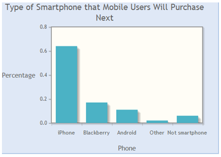
(1) Use the bar graph to find the appropriate probability model for the next phone choice of a randomly selected mobile phone user in Minneapolis.
| Phone Choice | iPhone | Blackberry | Android | Other | Not a smartphone |
|---|---|---|---|---|---|
| Probability | UcNnR32RxSVOsJiC5axSJ3kh4CelfY0Qtml2koBaSz5K+FCT | RR/ou5ENMEoEc1CjLhXUulcfAMFeE1ebKl3Ms7il4r8wYpLe | YvsU8+FCCQS8JpX4V8DdBjWmEwgzSPRNsdZOY79xJicSqr3M | s/BytNU7esKVCg3DBAd3spVOTx9JS//OASWaQYF62BXLKPtd | AGlCKw5hxAN4tz4U27woDSjg17mT+aw1v+E6vvWzQ9PEXQ0L |
(2) What is the probability that a randomly selected mobile phone user's next phone choice is not a Blackberry? ciWBmmEDWpcEuUvw
Correct.
(1)| Phone Choice | iPhone | Blackberry | Android | Other | Not a smartphone |
|---|---|---|---|---|---|
| Probability | 0.64 | 0.17 | 0.11 | 0.02 | 0.06 |
(2) P(not Blackberry) = 0.83
Incorrect.
(1)| Phone Choice | iPhone | Blackberry | Android | Other | Not a smartphone |
|---|---|---|---|---|---|
| Probability | 0.64 | 0.17 | 0.11 | 0.02 | 0.06 |
(2) P(not Blackberry) = 0.83
6.1.1 Discrete Random Variable and Their Probability Models
Recall that in Chapter 5 we defined a random variable as a numerical variable with values that result from the outcomes of a random experiment. We gave as an example the number of boys in a three-child family. This is a discrete random variable because we can make a list containing all the possible outcomes. In this case, the possible outcomes are 0, 1, 2, and 3.
In Chapter 7, we will discuss continuous random variables, which are variables that can have any value within an interval of numbers. Continuous random variables have infinitely many values, which cannot be listed. An example of a continuous random variable is the speed of cars passing a certain milepost on I-70 in rural Missouri. According to Missouri state law, that variable can take on any value between the minimum highway speed of 40 miles per hour and the maximum highway speed of 70 miles per hour. (Of course, if you are willing to risk getting a ticket, you may drive your car less than 40 or more than 70 miles per hour.)
The point here is that it is not possible to list all the possible speeds a car could be traveling. Any speed, measured to any number of decimal places, is a legitimate value for this variable.
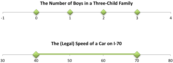
How can we decide whether a random variable is discrete or continuous? There are two ways to think of this.
- A discrete variable is something we count, while a continuous variable is something we measure. We count the number of children in a family, but we measure the speed of a car.
- A graph of the values of a discrete variable consists of dots spaced out on a number line, while a graph of the values of a continuous variable is connected. Using the children and speed examples, we have the following graphs:
Question 6.2
Determine if each of the following experiments produces a discrete random variable.
tsZWwutpaiAek8WyjAwx1KCBA8SY2e1ZThKxBpIlFa63dm8MEBZ7LknAw3sKj21Se7i43u9NFzKhiq/xoQ3T/fqYSS8d/mLCmtKQWdJ0aJ6QU77NwIzB63oGSOrTJCErKjtxP4A+R9wXYd851HIsxD0hxcZbi7SJ1hMEP/CH6LwrZ3DVyrlZEKqhEK5DNSOYfoWXc94RQrLs8K2a/W+mB7An33UonsHt2T+2+5wPhrCwytFDFM65bC7X0ilohDGIQhelHygWrA6pT0WLeuKIo268uXM1VX04USzAwoKjGhHn4tqo3d0HhOb0haLBzIELE/Inhmin221C8Tyov9eEDFC+OAtjnNCVKrAsDiveb5ei8L0s0uo1EWNBK7vyyegs38o1lgw8eqTE2PoDkNRZiyjkZqY= IU7W/BaOXsgd4giC/GSem07agg5ZtF6qi1HDFhcpvnwYj4hnMkkVJCJQ7YlSu4X05L627dfo0VkwMOv59oRJNMaf8lnr4qt0jtV+Q9lmBRctsIcP1kNJ+yrK+UdxukMoBKLyyZ+4xdPwNHCadU4XeNtYzpL2ntDC9YfzcceCrqAsr/RAI5BcwEcNpIoPrdUpiLFDZiT6KqHwsTY5JjATFhiAUXLM3OHrJ4iVMDRr7yXinHQ0xBlBe9xdLVumUhTR22qyJf8YoA4qS5u7h4DWnVVfFUruH79xvTJAMWXZhX3mtUvsUhfrZtjWCrhNeCRuRDS3NgvuvE8xM+l+6Z1C8vFNmzjH1elKU9Ae6ez8d1c= fuHrCNbyRaxsRrrF+YBZsruWaURPfd7HVLMH5a2boCaANH8iUFBTrnyMHo3PQMD2iXttQ4PZP6eaJAUdAlpxUU4kItsSeu0/AwdPZLoSupDoOdu2fNeobaX+vwsZZBhrlEewHQr7lUu38WFGEF91jlRsWYdmQqA9HVvKxP5VlX4wzo9uRAm1/Uf0QhcekwssPeaVgsjmvU4NYeFy1NJ3LAD91xcmFbY3WnC959ZO18Ho8ppPazblP/Hdefh9vZbb+SRcd/U1Tt4MprOOqZ6mbQfqFMwct61CvKEqSt52JgPF1ylSaKGk/iFlUOucHKBjHJk49yZOUldEsmYzQ54jx/30wawSkgbe9odH9r/44D8rXIoS l/Qg3BmIgaHxvC4gJ3tCGtELH2lO4cBVkKxz7o0DJhPG5fneePfFTkLryYhUxqTnbnO8HJ5VLtRa0By9hfV0QCNy280mMmwj8IfpTvrD2LAz4JRVVl5h8Sha9unNRmkGW9At87txa2eKLxBrUFdh+jymRwE9i3F5D3LDwhRr7F503fTyxpSS8McCVE1mZTUk8Y71vntrYZcBdelhR4fGwLbhBE9xGt45ltN2j07+uU1+hM2IvoHnetPjZyCSPO1mHFaw25pFqcpDbYgcABy8bUzB6b716+5pGwWPHccFiwYK6h7pzMkBi+JKPza5BhUlw39tcOrPQwdNeRGo0Ahr1AON/X8= mgbs+e0uOWyfHNmY4PFU7rcw8PxjhepOBoIT5QQB0+T166Ilhrb0jIZAWL0U/LcvFNLMW4iA7WZQiOEp+JMrbDz7A+i6G2LymISBX6CJEoHvrEonJQe9ZiwJmp/0cymLVq4NGz6n5/XzpjgjPvJyaV2/dgOyJx0llGbDbbWEGeYkES1kTpXuo9zP+TIDezljwxvZrpNl0hQH0YCf45AsgqUgjfPHP+KfRP4ZUAWZv1+M0rZZ/ggN5xUADcAi8ceBb5ewfyFLi7DlPgH15DW+UrNRqeDymeRecQSd3dTSrH/I/GlUllI1r+FrWiQrTQFkJ6KqWw+Z8uLtujmnbu2ekwz1c8Dj9mtTKThnHBwfRD1w2+Bj35eYTvUGHJb6jkKm(1) This experiment does not produce either type of random variable, because the outcomes of the experiment are not numerical.
(2) This experiment produces a random variable, but it is continuous rather than discrete.
(3) This experiment produces a discrete random variable.
(4) This experiment produces a discrete random variable.
(5) This experiment produces a random variable, but it is continuous rather than discrete.
(1) This experiment does not produce either type of random variable, because the outcomes of the experiment are not numerical.
(2) This experiment produces a random variable, but it is continuous rather than discrete.
(3) This experiment produces a discrete random variable.
(4) This experiment produces a discrete random variable.
(5) This experiment produces a random variable, but it is continuous rather than discrete.
Because we can list each outcome for a discrete random variable, we can construct a table to display its probability model. Let’s look once again at the tree diagram we made in Chapter 5 for the genders of children in a three-child family. At the end of each branch, we can show the family summary (by gender) and the number of boys.
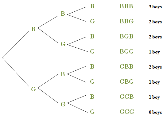
We can see that, if we repeatedly select a three-child family at random, in the long run, one-eighth of those families will have no boys at all. Thus the probability of no boys in a 3-child family is 1/8 or 0.125. Proceeding in the same way for 1, 2, and 3 boys, we obtain the following probability model for the number of boys in a three-child family.
| Number of Boys | 0 | 1 | 2 | 3 |
|---|---|---|---|---|
| Probability | 0.125 | 0.375 | 0.375 | 0.125 |
The decimals in this table are exact values corresponding to the fractions 1/8 and 3/8. To be valid, a discrete probability model must satisfy two conditions: (1) each probability is between 0 and 1 inclusive, and (2) the sum of the probabilities for all outcomes is 1. This model satisfies those conditions.
Suppose that we wanted to use this model to find the probability that a three-child family has more than 1 boy. Because having (exactly) 2 boys and (exactly) 3 boys are disjoint events, the probability of either 2 boys or 3 boys is the sum of their separate probabilities. So, P(2 boys or 3 boys) = P(2 boys) + P(3 boys) = 0.5.
Question 6.3
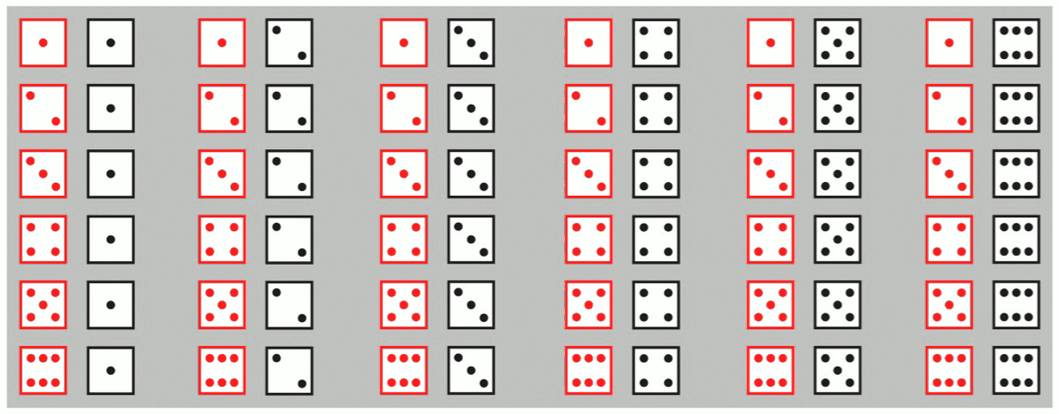
(1) Use the graphic below to complete the table giving the probability model for the sum of the numbers on the dice when two dice are rolled. Fill in the numerator for each probability fraction.
| Sum | 2 | 3 | 4 | 5 | 6 | |
|---|---|---|---|---|---|---|
| Probability | 0VV1JcqyBrI=/36 | XvVM00l89Is=/36 | 607M7xmPORU=/36 | h4XZagboIgc=/36 | DYU2tVvtzEQ=/36 | |
| Sum | 7 | 8 | 9 | 10 | 11 | 12 |
| Probability | yBhAQ+3VvjM=/36 | DYU2tVvtzEQ=/36 | h4XZagboIgc=/36 | 607M7xmPORU=/36 | XvVM00l89Is=/36 | 0VV1JcqyBrI=/36 |
(2) Use your model to determine the probability that you roll a 9 or higher on your first roll in a game of Monopoly. Pz2PEfhsNWI=/36
Correct.
(1)| Sum | 2 | 3 | 4 | 5 | 6 | 7 | 8 | 9 | 10 | 11 | 12 |
|---|---|---|---|---|---|---|---|---|---|---|---|
| Probability | 1/36 | 2/36 | 3/36 | 4/36 | 5/36 | 6/36 | 5/36 | 4/36 | 3/36 | 2/36 | 1/36 |
(2) These probability values are the exact, unreduced fractions. It is easy to confirm that the sum of these fractions is 1. P(Sum ≥ 9) = 4/36 + 3/36 + 2/36 + 1/36 = 10/36.
Incorrect.
(1)| Sum | 2 | 3 | 4 | 5 | 6 | 7 | 8 | 9 | 10 | 11 | 12 |
|---|---|---|---|---|---|---|---|---|---|---|---|
| Probability | 1/36 | 2/36 | 3/36 | 4/36 | 5/36 | 6/36 | 5/36 | 4/36 | 3/36 | 2/36 | 1/36 |
(2) These probability values are the exact, unreduced fractions. It is easy to confirm that the sum of these fractions is 1. P(Sum ≥ 9) = 4/36 + 3/36 + 2/36 + 1/36 = 10/36.
6.1.2 Expected Value of a Discrete Random Variable
Many people play the lottery every week in hopes of striking it rich. If you buy the occasional lottery ticket, you may not expect to win. The ticket is a lark. But if you buy a ticket every week, do you expect to make money in the long run? For example, what would the average return be on a $2 Powerball lottery ticket?
Figure 6.3 shows the odds of winning the various prizes, as reported by the Multi-State Lottery Association.
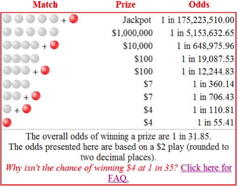
The value of the grand prize changes depending on the number of tickets sold and how long it has been since someone has won. Also, the odds of winning the grand prize are less than 1 in 100,000,000, in other words, very small. For the purposes of our discussion, we will not consider that prize.
The values for the other prizes remain the same from week to week. The table below converts the odd for winning a prize to its corresponding probability (reported to one significant digit).
| Prize | Probability of Winning |
|---|---|
| $1,000,000 | 0.0000002 |
| $10,000 | 0.000002 |
| $100 | 0.0001 |
| $7 | 0.004 |
| $4 | 0.03 |
Can we convert this table into a probability distribution? It should be clear that when we add up all these probabilities, we get a value far less than one. So what are we missing?
Because you might not win at all, what is missing is the probability that you win nothing.
If we let the random variable X be the dollar amount of the winnings, then P(0) = P(not winning a prize) = 1- P(winning a prize). Therefore,
P(0) = 1 – (0.0000002 + 0.000002 + 0.0001+ 0.004 + 0.03) = 1 – 0.0373022 =0.9659, and the probability distribution for X is given in the table below.
| X | $0 | $4 | $7 | $100 | $10,000 | $1,000,000 |
|---|---|---|---|---|---|---|
| P(X) | 0.9659 | 0.03 | 0.004 | 0.0001 | 0.000002 | 0.0000002 |
Yet our question remains what is the average return on a $2 Powerball lottery ticket? Let’s look first at what not to do--simply average the prize amounts. The average of the prize amounts is
\( \frac{0 + 4 + 7 + 100 + 10,000 + 1,000,000}{6} = \frac{1,010,111}{6} = 168,251.8333 \) (or $168,251.83 rounded to the nearest cent).
If it were possible to win an average of $168,251.83 on $2 Powerball lottery tickets over many, many weeks, we’d all be buying tickets and waiting for the cash to roll in.
What we neglected to consider is that all these outcomes are not equally likely. To find the average winnings, we must take into account how likely each prize is to occur. The average value of X is found by multiplying each prize by its probability, then adding the resulting numbers:
0(0.9659) + 4(0.03) + 7(0.004) + 100(0.0001) + 10,000(0.000002) + 1,000,000(0.0000002) = 0.378 or $0.38, correct to the nearest cent.
If we spend $2 dollars every week on a lottery ticket, on average we win 38 cents a week; that is, on average we actually lose $1.62. In the long run, this is not a good bargain.
Because this average (or mean) value represents what we expect to happen in the long run, we call it the expected value of the random variable. The expected value of a random variable is the sum of the products obtained by multiplying each value of the random variable by its probability.
In formula form, if we let x represent each of the particular values of the random variable X, then the expected value of X is
\( \mu_{x} = \sum x \cdot P(x)\)
Question 6.4
Consider X to be the number of dog-owning households in a random sample of five U.S. households. The table below gives the possible values for the random variable X, and the probability associated with each value.
| X | 0 | 1 | 2 | 3 | 4 | 5 |
|---|---|---|---|---|---|---|
| P(X) | 0.10 | 0.29 | 0.34 | 0.20 | 0.06 | 0.01 |
Find the expected value of the random variable X: 5/4hIfjM3Is=
μx = 0·0.10 + 1·0.29 + 2·0.34 + 3·0.20 + 4·0.06 + 5·0.01 = 1.85
μx = 0·0.10 + 1·0.29 + 2·0.34 + 3·0.20 + 4·0.06 + 5·0.01 = 1.85
You may be interested to know that in addition to finding the average for the random variable X, we can also find its standard deviation. We use the formula
\( \sigma _{x} = \sqrt{\sum (x-\mu_{x})^2} P(x)\)
which looks pretty horrible at first glance. But if we take a look under the square root symbol, we see that we are again adding up a set of products. The first factor of each product is the square of the difference (deviation) between each value and the mean, and the second factor is the value’s probability.
This is not a calculation you would want to do by hand, but it is useful to see its similarities to both the population standard deviation (done in Chapter 3) and the expected value done above.
As we saw in Chapter 3, the standard deviation provides a measure of how far the data points are dispersed from the mean. Here is a graph of the probability model for the sum of the numbers on the dice when two dice are rolled.
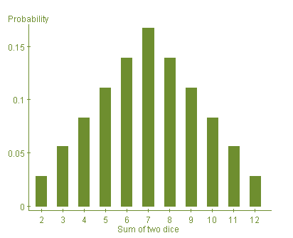
In this example, μx = 7 and σx = 2.415. How should we interpret the standard deviation in this instance? Because this distribution is bell-shaped, we can apply the Empirical Rule from Chapter 3 to interpret the mean and standard deviation in the context of this problem.
Recall that the Empirical Rule tells us that there is approximately a 95% chance that the sum of the two rolls will be within 2 standard deviations of the mean. Here are the calculations:
μx - 2σx = 7 - (2·2.415) = 2.17 and μx + 2σx = 7 + (2·2.415) = 11.83.
Therefore about 95% of the time we expect that the sum of the two rolls will be between 2.17 and 11.83.
Many common situations involve discrete probability models. In this section, we have discussed properties that apply to all such models. There are many specific types of discrete probability models, each with its own interesting properties and applications. In the next section, we will present a particular model that appears in many different settings.