8.1 Confidence Intervals for a Population Proportion
Public opinion polls, such as those conducted by the Gallup organization or the Washington Post, are typically used to measure the behavior or opinions of people on a wide array of topics. These organizations draw conclusions about a large population based on a relatively small sample selected from it. How are they able to use a small sample to draw a broad conclusion? Wouldn’t they get a different result if they used a different sample?
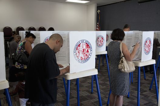
Understanding why we can rely on polling results from reputable organizations requires that we understand the variability of samples taken from the same population. Consider the U.S. presidential election of 2012. The table below (from www.realclearpolitics.com) shows the final poll results from a number of different polling organizations, along with the actual results (Obama 51.1%, Romney 47.2%).
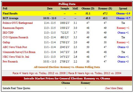
Notice that all of these polls were taken at roughly the same time, within a week of the election. All of the polls surveyed likely voters (LV), with sample sizes ranging from 693 to 2709. The percentage of participants favoring Barack Obama varied from a low of 47% to a high of 50%. Why were the results different? The simple answer is that the various polls questioned different individuals. Although all samples contained likely voters, the voters who were actually surveyed differed from poll to poll.
Let’s take another minute and look at the sample sizes. The pollsters were interested in studying the population of all likely voters. This population includes approximately 130 million people, yet in each sample only a tiny fraction (between 0.00005% and 0.0002%) was sampled. How can we have any confidence in the accuracy of these polling results when such a small percentage of the population was polled? As we’ll see shortly, samples of these sizes are just fine, provided that each sample was collected randomly.
Nate Silver is a statistician and journalist who began his career as an economics consultant while pursuing his hobby of analyzing Major League Baseball performance. He began political forecasting in 2008, and in 2012 correctly predicted the outcome of the presidential election in all 50 states and the District of Columbia. After the election Newsweek reported on the effect of his quantitative methods on political reporting.
Before we go any further, let’s clarify the notation we will use in our discussion. We will use \(p\) to denote the proportion of the population possessing a certain characteristic, while \(\hat{p}\) (called p-hat) represents the proportion of a sample possessing the characteristic. That is, if we let \(x\) represent the number of individuals in the sample of size \(n\) who possess the characteristic, \(\hat{p} = \frac{x}{n}\). Recall that in our discussion of binomial probability, we referred to possessing the characteristic as success. So \(\hat{p}\) represents the proportion of successes in the sample.
In the election example, \(p\) represents the proportion of all voters who voted for Barack Obama, while each of the sample proportions of those favoring Obama prior to the election is represented by \(\hat{p}\).
The polling results in Figure 8.1 display sampling variability, the variation that occurs in a sample statistic, like \(\hat{p}\), when different samples from the same population are selected. This variability is sometimes referred to as sampling error, which makes it sound like there was some mistake in the process. However, regardless of the care you take in selecting a sample (and recall that a simple random sample is the gold standard for our purposes), sample statistics vary because samples are different. Sampling variability is not a mistake that needs correction; it is a natural part of the process of random sampling. It is a fact of statistical life, but one that must be accounted for when we want to draw a conclusion about a population parameter based on the value of a single sample statistic.
8.1.1 The Sampling Distribution of a Sample Proportion p̂
The goal we have in mind is to draw a conclusion about \(p\) when we know the value of \(\hat{p}\) from only a single sample. (We don’t want to take multiple samples, because this involves additional time and usually more money as well.) So we would like to know what the set of all possible \(\hat{p}\)’s looks like. We call the distribution of these \(\hat{p}\)’s the sampling distribution of \(\hat{p}\).
Suppose that we select every possible sample of size \(n\) from the population of interest, and calculate the proportion \(\hat{p}\) having the desired characteristic in each sample. As long as the sample size is large enough, we would find that these sample proportions were approximately normally distributed, with their mean equal to the population proportion \(p\) and their standard deviation equal to \(\sqrt{ \frac{p(1-p)}{n}}\).
We say that the sampling distribution of \(\hat{p}\) is approximately normal with \(\mu_{\hat{p}} = p \) and \(\sigma_{\hat{p}} = \sqrt{ \frac{p(1-p)}{n}}\). This approximation can be used whenever \(n\) and \(p\) are such that the number of successes (\(np\)) and the number of failures \((n(1-p))\) are each at least 10.

Statistical software can give us a sense of what the distribution looks like by simulating such sample proportions and constructing a histogram of their values.
The notation gets a bit complicated here. The mean of the sampling distribution, \(\mu_{\hat{p}}\), is a \(\mu\) because it is the average of all the possible \(\hat{p}\)’s. We use the subscript \(\hat{p}\) to remind us that this is an average of all possible \(\hat{p}\) values. So \(\mu_{\hat{p}}\) is the mean of a population that consists of sample proportions. We use the corresponding sigma notation, \(\sigma_{\hat{p}}\), for the standard deviation of the sampling distribution of \(\hat{p}\).
For our election example then, if we chose samples of size 1000, then \(np=1000 \times 0.511 = 511\) and \(n(1-p)=1000 \times (1-0.511) = 499\). Since the number of successes and the number of failures are each at least 10, the sampling distribution of \(\hat{p}\), the sample proportion of voters favoring Obama, would be approximately normal, with mean \(\mu_{\hat{p}}=0.511\) and standard deviation \(\sigma_{\hat{p}}=\sqrt{\frac{0.511(0.489)}{1000}}\approx0.016\).
It is important to remember that if we were able to select every possible sample of size 1000 from the population of all those who voted for president in 2012, the distribution of these sample proportions would be approximately normal, with a mean of 0.511 and a standard deviation of 0.016.
The graph below shows the distribution of 2000 sample proportions (each with a sample size of \(n=1000\)) simulated from the Obama results.
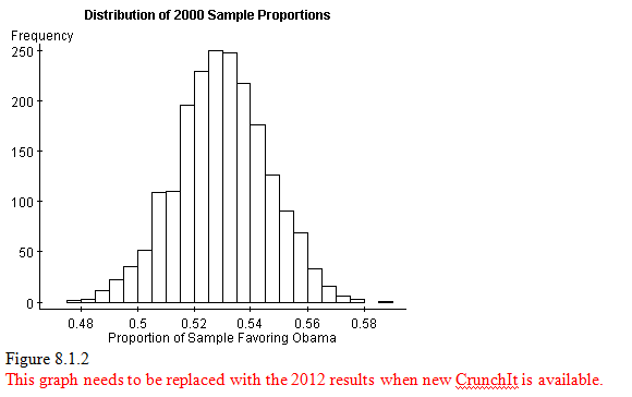
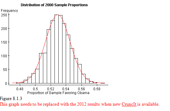
We can see that the histogram is symmetric and bell-shaped, with center at about 0.51. The figure shown below includes the appropriate normal curve (\(\mu_{\hat{p}}=0.511\) and \(\sigma_{\hat{p}}=0.016\)). We see a very close correspondence between the histogram and the normal curve, even though 2000 samples, each of size \(n=1000\), is a very, very small fraction of all the possible samples from this population.
Please review the whiteboard "Sampling Distribution of Sample Proportion."
Question 8.1
Suppose that simple random samples of size 500 are taken from the population of 2012 presidential voters.
Use the fact that 47.2% of those who voted in the 2012 Presidential election favored Mitt Romney to describe the sampling distribution of \(\hat{p}\), the proportion of the sample favoring Mitt Romney. Round the values for \(\mu_{\hat{p}}\) and \(\sigma_{\hat{p}}\) to three decimal places.
Rounded to 3 decimal places, the sampling distribution of \(\hat{p}\) is approximately 67oA3rZXG43lk5wa, with \(\mu_{\hat{p}}\) = JR5+jfMLUsrL3QlA8Dr0cg== and \(\sigma_{\hat{p}}\) = YhvdoTMV1mJRnG8K.
Question 8.2
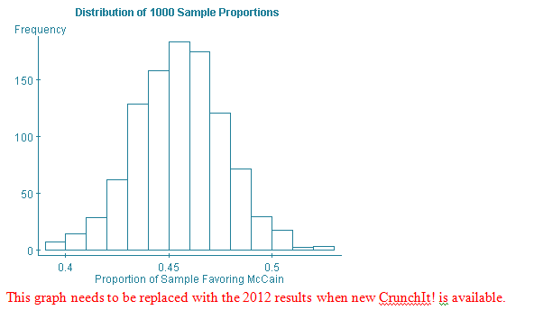
Use your answer to the first question and the Sample Proportion applet to select 1000 sample proportions. Make a histogram of the proportions, and describe its shape and center.
The histogram is 3d4cmnZkZU8=-shaped. The center is between t/tkDeHYlkREHZ+lmG1zILl5myPPLWoS2n0UdYiS8fA= and OQOJjG96LXB+AFqxNuz4FWXx8YFEPR0AiXX0/Q2WJJ4=. (Round values to two decimal places.)
Correct. Histograms vary; one histogram is shown below. Histograms should be bell-shaped with a center between 0.47 and 0.48.
Incorrect. Histograms vary; one histogram is shown below. Histograms should be bell-shaped with a center between 0.47 and 0.48.
8.1.2 The Idea Behind Confidence Intervals
Because we know that the sampling distribution of \(\hat{p}\) is approximately normal, we can use the Empirical (68-95-99.7) Rule to describe the variability of the \(\hat{p}\)’s. For the sample proportions of voters favoring Obama, about
- 68% of all \(\hat{p}\)’s lie within 1 standard deviation of \(p\) (between 0.495 and 0.527).
- 95% of all \(\hat{p}\)’s lie within 2 standard deviations of \(p\) (between 0.479 and 0.543).
- 99.7% of all \(\hat{p}\)’s lie within 3 standard deviations of \(p\) (between 0.463 and 0.559).
Even with only 9 sample polls shown in Figure 8.1, we can see a good correspondence with the rule: 8 of the 9 (89%) of the \(p\)’s are within 2 standard deviations of \(p = 0.511\). It is nice to see, after the fact, that the \(\hat{p}\)’s behave the way that we expect them to.
When we select one sample at random from all the possible samples of a certain size, we calculate the sample proportion (for the characteristic being studied) for that sample. About 95% of the time, that sample proportion will be within 2 standard deviations of the true (but typically unknown) population proportion. So, 95% of the time, the true (but typically unknown) population proportion is within 2 standard deviations of whatever sample proportion we have obtained from our random sample selection.
This is why we can depend on the poll results. 95% of the time, the unknown population proportion will be within 2 standard deviations of whatever sample proportion results after our random sample selection. So the polling organization reports the sample proportion, and then gives us a (roughly) 2-standard-deviation margin of error within which they expect the true proportion to fall. And they tell us they are 95% confident of their result.
Because of differences in sample sizes and sample proportions in the 2012 election polls, the margins of error (MoE in Figure 8.1) differ from poll to poll. In each and every case, however, the true proportion of votes received by Obama falls within the interval (sample proportion – margin of error, sample proportion + margin of error). For example, the Pew Research poll had a sample proportion favoring Obama of 0.50, with a margin of error of 2.2%. According to this poll, then, the true proportion voting for Obama is likely to fall between 0.478 and 0.522. We see that the true proportion of votes for Obama (0.511) is indeed within the interval.
8.1.3 Confidence Intervals for a Population Proportion
Now that we see the big idea behind confidence intervals, we can look more closely at the mathematical details. In general, a confidence interval is of the form estimate ± margin of error. The estimate is a sample statistic; the margin of error is determined by an estimate of the standard deviation of the sampling distribution and how frequently we are willing to be wrong. The sample statistic is easy to find and to understand. The two values that determine the margin of error are not.
Calculating the standard deviation of the sampling distribution requires that we know the true population proportion \(p\), since \(\sigma_{\hat{p}}= \sqrt{\frac{p(1-p)}{n}}\). But \(p\) is exactly what we are trying to determine. So the best we can do is to use \(\hat{p}\) to estimate \(p\). When we do that, we create what we call the standard error of the sample proportion \(SE_{\hat{p}}= \sqrt{\frac{\hat{p}(1-\hat{p})}{n}}\).
The standard error of the sample proportion, \(SE_{\hat{p}}= \sqrt{\frac{\hat{p}(1-\hat{p})}{n}}\), is therefore an estimate of the standard deviation of the statistic, \(\sigma_{\hat{p}}= \sqrt{\frac{p(1-p)}{n}}\).
How frequently we are willing to be wrong requires some thought. We know from the Empirical Rule that if we created lots and lots of confidence intervals by starting with a sample proportion and going two standard deviations away from it in each direction, about 95% of all the intervals would contain the true population proportion. So 5% of them would not. The problem is that when we don’t have the true proportion in the first place, we don’t know if any particular interval is good or bad. And using \(SE_{\hat{p}}\) instead of \(\sigma_{\hat{p}}\) can make matters worse. The bottom line is, using this method means that we are willing to be wrong (and not know it) 5% of the time.
How willing you are to be wrong should depend on how serious the consequences of an error would be. While you are free to decide for yourself how often you are willing to be wrong, typically statisticians have settled on the percentages 10%, 5%, and 1%, which generate 90%, 95%, and 99% confidence intervals respectively. These percentages (90, 95, 99) are called the confidence levels of the intervals.
Because we use a normal model for the sampling distribution for a sample proportion, when we talk about how far to go out in terms of standard deviations or standard errors, we measure in \(z\)’s. In order to trap the true population proportion 90% of the time, we need a \(z\) of 1.645, while a \(z\) of 2.576 is required if we want the true proportion in our interval 99% of the time. Our rule of thumb value, \(z = 2\), for creating intervals containing the true proportion 95% of the time was a convenient approximation but is a bit larger than needed. The value of \(z\) for creating a 95% confidence interval is more accurately 1.960.
The values needed for generating particular confidence intervals are called critical values, and are designated by \(z^{*}\). The critical value is determined by the person who is calculating the confidence interval. The table below summarizes the critical values for the most common confidence levels.
| Confidence Level | Critical Value |
|---|---|
| 90% | z* = 1.645 |
| 95% | z* = 1.960 |
| 99% | z* = 2.576 |
Please review the whiteboard "Finding Confidence Interval z Values."
Now we can put everything together and create a formula for creating a confidence interval for the population proportion:
estimate ± margin of error
\(\hat{p}\pm z^{*}SE_{\hat{p}}\)
\(\hat{p}\pm z^{*}\sqrt{\frac{\hat{p}(1-\hat{p})}{n}}\)
Let’s try this formula on the Pew Research poll results for voters favoring Obama. They reported a \(\hat{p}\) of 0.50 and a sample size \(n=2709\). Then a 95% confidence interval is given by:
\(0.50\pm 1.96\times\sqrt{\frac{0.50(1-0.50)}{2709}}\)
\(0.50\pm 0.0188\)
Thus, if we round to two decimal places, we get approximately the margin of error that is in Figure 8.1. If we use the four-decimal-place value, we obtain an interval of 0.4812 to 0.5188, which again contains the true population proportion of 0.511.
Question 8.3
In the CNN/Research the sample proportion of voters favoring Mitt Romney was 0.49, with a sample size of 693. Use these data to find the margin of error for a 95% confidence interval for the true proportion of voters favoring Mitt Romney. Round your answer to four decimal places.
The margin of error is XeCE3WbEHWJLxI7UbKR2PQ==.
The margin of error is 0.0372, or 3.72%.
The margin of error is 0.0372, or 3.72%.
8.1.4 Building and Interpreting a Confidence Interval
Even though using the confidence interval formula requires only a small amount of calculation, we are ready to abandon it in favor of statistical software (and we will leave our election poll example behind as well).
A 2013 poll of 1006 adults living in the continental United States found that 61% of Facebook users have at some time voluntarily taken a break from using Facebook for a period of several weeks or more. Let’s use CrunchIt! to construct 90%, 95%, and 99% confidence intervals for the true proportion of Facebook users who have voluntarily taken a break from it for a period of several weeks or more.
To find a confidence interval, many versions of technology require that you know the number of successes \(x\) (the number of individuals in the sample having the desired characteristic) as well as the sample size. For this Gallup Poll, \(x\) is the number of people who have a Facebook account who have voluntarily taken a break from it at some time, and we can find it by calculating 61% of 1,006, which is roughly 614.
Table 8.2 shows the intervals calculated by CrunchIt! for various confidence levels.
| Confidence Level | Lower Limit | Upper Limit |
|---|---|---|
| 90% | 0.5851 | 0.6356 |
| 95% | 0.5802 | 0.6405 |
| 99% | 0.5707 | 0.6499 |
What do we find? The shortest interval, the one with the smallest margin of error, was the 90% confidence interval (0.5851, 0.6356). The longest interval was the 99% confidence interval (0.5707, 0.6499), because its margin of error was the largest. And the 95% interval was in the middle in terms of its length.
When we pause for a moment to consider this, it makes perfect sense. If we want to be 99% confident, we are willing to be wrong only 1% of the time, so we must include a wider set of possible values for \(p\) than if we are willing to be wrong 10% of the time. For many applications, a 95% confidence level strikes the right balance between not being wrong too often and not having too long an interval as an estimate.
Notice also that the sample proportion 0.61 is exactly in the middle of each interval. This is always the case, because this is how we build the interval. We use the sample proportion as a starting point and go \(z^{*}\) estimated standard errors to the left and to the right of this value. So if someone reported a confidence interval of (0.8220, 0.8580), you would know that the sample proportion \(\hat{p}\) would be the average of the interval’s endpoints, or \(\frac{0.8220+0.8580}{2}=0.8400\).
Please review the whiteboard "Confidence Interval to Estimate p."
Question 8.4
The cost to run the Olympics is huge. A BBC Poll of 3,218 adults in the United Kingdom in July 2013 found that 69% believed that the 8.77 billion pound cost (approximately 13.5 billion U.S. dollars) of the London 2012 Olympics was worth the cost. Find 90%, 95%, and 99% confidence intervals for the true proportion of British adults who believed the high cost of the 2012 Olympics was worth it. Write each answer in interval form, using four decimal places.
(a) The 90% confidence interval for the true proportion of British adults who believed the high cost of the 2012 Olympics was worth it is (4HtXQ07AbFUNeqjc2ztArw== , wUlNdmG+T9SR20w0+6QZFg==).
(b) The 95% confidence interval for the true proportion of British adults who believed the high cost of the 2012 Olympics was worth it is (4ya1f6vZ8gkisWkAVNaAtw== , w4Q6fXhNdRS8kuTs/jJgCg==).
(c) The 99% confidence interval for the true proportion of British adults who believed the high cost of the 2012 Olympics was worth it is (pp+agWsp4PBU0KggvakkgQ== , ZuQ9h3uRiE7Rq5eYDhw9Fg==).
Correct. Using 4-decimal-place values, the 90% confidence interval for the true proportion of British adults who believe the high cost of the 2012 Olympics was worth it is (0.6765, 0.7033).

The 95% confidence interval is (0.6739, 0.7059).

The 99% confidence interval is (0.6689, 0.7109).

Again we see the pattern of the longer intervals being associated with higher confidence levels.
Incorrect. Using 4-decimal-place values, the 90% confidence interval for the true proportion of British adults who believe the high cost of the 2012 Olympics was worth it is (0.6765, 0.7033).
The 95% confidence interval is (0.6739, 0.7059).
The 99% confidence interval is (0.6689, 0.7109).
Again we see the pattern of the longer intervals being associated with higher confidence levels.
Now that we have taken care of the (relatively) easy matter of building a confidence interval, we turn our focus to the more difficult question of correctly interpreting such an interval. Consider again the 90% confidence interval (0.5851, 0.6356) for the true proportion of American adults with a Facebook account who have voluntarily taken a break from Facebook at some point. We will say that we are 90% confident that the true proportion of American adults with Facebook accounts who have voluntarily taken a break from it at some point is between 0.5851 and 0.6356. Or, if you prefer percentages, and round numbers, we are 90% confident that between 59% and 64% of American adults with Facebook accounts have voluntarily taken a break from it at some point.
But what does that actually mean? Our confidence level (90% in this case) represents a probability, but not in the way you might think. Recall that probability refers to the long-run behavior of phenomena whose behavior in the short term is the result of chance. To build our interval we started with a single sample proportion--a proportion determined from a randomly chosen sample. All we know is that if we repeated this process over and over by taking many random samples, 90% of the intervals we obtained would contain the true population proportion. Thus, our confidence rests with the method we use to construct the interval, not with any particular interval we construct.
Can we say that 90% of the time the true proportion lies between 0.5851 and 0.6356? Definitely not. The true proportion is a number, unknown but not changing. It doesn’t move around, sometimes landing between 0.5851 and 0.6356, and sometimes not. The real value of \(p\) is either in that interval or it is not. Is there any way for us to tell? Unfortunately, no. The best we can say is that we are using a method that traps the true proportion in 90% of the intervals calculated.
For the very same reason, we cannot say that the probability that the true proportion lies between 0.5851 and 0.6356 is 0.90. It is important for you to remember that the proportion we are trying to estimate is some fixed number between 0 and 1; it is just not known to us. When we take different samples, we get different intervals. In the very long run, 90% of the 90% confidence intervals do contain the true population proportion we are attempting to estimate.
The table below shows twenty 90% confidence intervals generated from a population with true proportion of successes \(p = 0.7\). (Values for \(\hat{p}\) and interval endpoints have been rounded to 2 decimal places.)
| \(\hat{p}\) | 90% confidence interval | Is \(p=0.7\) in interval? |
|---|---|---|
| 0.72 | (0.65, 0.79) | Yes |
| 0.76 | (0.69, 0.83) | Yes |
| 0.63 | (0.55, 0.71) | Yes |
| 0.69 | (0.61, 0.77) | Yes |
| 0.73 | (0.66, 0.80) | Yes |
| 0.71 | (0.64, 0.78) | Yes |
| 0.64 | (0.56, 0.72) | Yes |
| 0.75 | (0.68, 0.82) | Yes |
| 0.64 | (0.56, 0.72) | Yes |
| 0.75 | (0.68, 0.82) | Yes |
| 0.64 | (0.56, 0.72) | Yes |
| 0.65 | (0.57, 0.73) | Yes |
| 0.68 | (0.60, 0.76) | Yes |
| 0.71 | (0.64, 0.78) | Yes |
| 0.61 | (0.52, 0.69) | No |
| 0.67 | (0.59, 0.75) | Yes |
| 0.70 | (0.62, 0.78) | Yes |
| 0.75 | (0.68, 0.82) | Yes |
| 0.67 | (0.59, 0.75) | Yes |
| 0.74 | (0.67, 0.81) | Yes |
| 0.80 | (0.73, 0.87) | No |
| 0.73 | (0.66, 0.80) | Yes |
There are several things to notice here. First, as it must, each \(\hat{p}\) lies exactly in the middle of its confidence interval. Second, because \(\hat{p}\)’s are different, the intervals are not all the same length. Third, 90% of our twenty 90% confidence intervals do contain the true population proportion \(p = 0.7\), while 10% do not. We were fortunate that things turned out this way, since looking at twenty confidence intervals hardly qualifies as the very long run. But these intervals demonstrate that the confidence we express is indeed in the process rather than the outcome. Had we selected just a single sample at random, we could have obtained one with \(\hat{p}\) of 0.80. If we had gotten \(\hat{p}=0.80\), the interval we created would not contain the true population proportion, and, unhappily, we would not know that.
So here is our advice about interpreting a confidence interval about a proportion:
- When you are asked to give a confidence interval, say “We are (whatever)% confident that the true proportion of (whatever you are trying to estimate) lies between (your lower bound) and (your upper bound).”
- When you are asked what the confidence level means, say “If we took random samples many times, and constructed a (whatever)% confidence interval based on each sample proportion, we would get many different intervals. About (whatever)% of those intervals would actually contain the true proportion of (whatever you are trying to estimate).”
If you say these sentences to yourself each time you construct a confidence interval, you will be less likely to misinterpret your intervals. Here is what you should take away from this discussion: When we report a 90% confidence interval, we mean that we have used a method that produces intervals containing the true population proportion 90% of the time in the long run. Our confidence lies in the long term dependability of the process rather than in any one particular interval. (And, of course, similar statements apply to intervals of any other level of confidence.)
8.1.5 Confidence Intervals -- Important Conditions
Now that we have looked at why we want to create a confidence interval, how to build one, and what the resulting interval means, it is time to consider when it is appropriate to do so. In order for us to use a normal probability model for the sampling distribution of \(\hat{p}\), the following conditions are required:
- The data come from a simple random sample from the population of interest.
- Individual measurements (success or failure) are independent.
- The sample size is no larger than 10% of the size of the population.
- The sample results include at least 10 successes and 10 failures.
In practice, it is very difficult, if not impossible, to guarantee that all these conditions are met. So we must do our best to explain why we believe our sample is good enough to use a confidence interval to estimate a population proportion.
As we shall see throughout our study of statistical inference, the most important condition is that the data come from a simple random sample from the population. If your sample is not truly a simple random sample, you must be able to explain why it is a close enough approximation to one to make your inference OK. If you grab a bag of M&M’s off the shelf of your local grocery store, does that bag constitute a simple random sample of all M&M’s? Was random chance responsible for its selection? Were all samples containing the same number of M&Ms equally likely to be chosen? The answers to these questions are no, no, and no. But, given quality controls on the production and distribution of M&Ms, it is reasonable to assume that your bag looks pretty much like a simple random sample.
That is quite a bit different from doing an opinion survey at your local shopping mall at 10:00 AM on a Tuesday morning. Here you are clearly dealing with a convenience sample, and are more likely to over-represent the opinions of older adults. The point is, unless you believe that your sample approximates a simple random sample, you should not use these inferential techniques.
The independence condition requires that data values are not related to each other. If you phone a simple random sample of people to ask their opinions, it is reasonable to believe that one person’s opinion is not affecting another’s. However, if you select a simple random sample of individuals, but interview them at the same time in the same place, one person’s opinion could very well be influenced by the opinions of others.
Even for non-human samples, if the characteristic studied is the presence of a contagious disease or a production defect, the selection of individuals closely related in space or time may suggest a lack of independence. In such a case, if our sample is random, we are more likely to be confident that the independence condition is met.
The last two conditions, concerning sample size and numbers of successes and failures are fairly easy to check. We generally know at least the relative size of the population, so we can choose a sample that is no more than 1/10 that size. And once we have the sample data, we verify that successes (\(n\hat{p}\)) and failures (\(n(1-\hat{p})\)) are at least 10.
Question 8.5
Smartphone adoption among American teens has increased dramatically over the past several years. A recent Pew Internet and American Life Project poll of 802 American teens between the ages of 12 and 17 in July 2013 found that 47% own a smartphone.
(a) Check that the conditions to construct a 95% confidence interval are satisfied:
- The techniques used by the pollsters creates a sample that pvTVwSmc4FEhGUIiyxNaevXT+GAvaC/V/3g8rdd3FeZgPvtn0h6Utg== a simple random sample from the population of all American teens.
- Individual responses EfVnTmSox3wG8cSeYInsEk0ImU4= independent.
- The sample size V4pWDsvrK/09a/S8Xc00Yg== larger than 10% of the size of the population.
- The sample results eOfHEABA+NwQ/d092RN10qtTu/E2otluIHD9J9vKqZE= at least 10 successes and 10 failures.
(b) Rounded to four decimal places, the 95% confidence interval to estimate the percentage of all American teens that own a smartphone is (zDdB12OILeVt1jxkNbujoQ== , 8kH8+Yx/14wuDac6mTOfVQ==).
(c) We are 95% confident that the percentage of kmdy93a8hDajkpT191GAO/IOz1JFftHUmE1J49Vp+3EqNzFzSdZWIUsbdJz0iIhUP7ah5VY4TTh4ZuCImNwSKbE0TGEZhjzf1w5i98d7rOePXEdBk9RrIdwaUZGYqrOc that own a smartphone lies between DxnlX4coZmM=% and fwIPnBkWdu4=%. Round any values to the nearest whole percent.
Correct.
(a) The techniques used by the pollsters to select a sample creates one that approximates a simple random sample from the population of all American teens. Individual responses are independent. The sample size is no larger than 10% of the size of the population. The sample results include at least 10 successes (\(0.47\times802=376.94\)) and 10 failures
(\(0.53\times802=425.06\)).
(b) (0.4355, 0.5046)
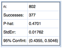
(c) We are 95% confident that the percentage of all American teens that own a smartphone is between 44% and 50%.
Incorrect.
(a) The techniques used by the pollsters to select a sample creates one that approximates a simple random sample from the population of all American teens. Individual responses are independent. The sample size is no larger than 10% of the size of the population. The sample results include at least 10 successes (\(0.47\times802=376.94\)) and 10 failures
(\(0.53\times802=425.06\)).
(b) (0.4355, 0.5046)
(c) We are 95% confident that the percentage of all American teens that own a smartphone is between 44% and 50%.
8.1.6 Choosing a Sample Size
When you look at popular opinion polls, such as the Gallup Poll, you may wonder about the choice of sample sizes. In the election polls we considered in Figure 8.1, we see sample sizes like 1417, 712, and 2345. Why not 1000, 700, and 2500? These seem like nicer numbers to us.
The NPR story U.N. Reports 35,000 Iraqi Civilians Killed in 2006 describes how different methods of data collection generate different estimates of deaths. Pay particular attention to the discussion about how sample size affects the length of the confidence intervals.
Sample sizes are chosen so that the confidence intervals created have a certain confidence level and a specific margin of error. Pollsters seem to prefer a margin of error in the range of 0.02 to 0.03 when estimating a population proportion. In order to obtain that kind of margin of error and still retain a (typically) 95% confidence level, the pollster works backward to find the smallest sample size that produces that margin of error. (He or she does not want a sample any larger than necessary because larger samples are more expensive, in terms of both time and money.)
Where does the margin of error come from? If we return to our confidence interval formula \(\hat{p}\pm z^{*}\sqrt{\frac{\hat{p}(1-\hat{p})}{n}}\), we see that the margin of error (MoE) is represented by \(z^{*}\sqrt{\frac{\hat{p}(1-\hat{p})}{n}}\). If we know the MoE we want, we can find the needed sample size with some algebraic manipulation:
\(z^{*}\sqrt{\frac{\hat{p}(1-\hat{p})}{n}}=MoE\)
\(\sqrt{\frac{\hat{p}(1-\hat{p})}{n}}=\frac{MoE}{z^{*}}\)
\(\frac{\hat{p}(1-\hat{p})}{n}=\big(\frac{MoE}{z^{*}}\big)^2\)
\(\frac{n}{\hat{p}(1-\hat{p})}=\big(\frac{z^{*}}{MoE}\big)^2\)
\(n=\hat{p}(1-\hat{p})\big(\frac{z^{*}}{MoE}\big)^2\), with MoE expressed in decimal form, and \(n\) rounded up to the next whole number.
While the process of obtaining it looks complex, the resulting formula isn’t too hard to use. The only difficulty comes in deciding what to use for \(\hat{p}\). Remember that we are using the formula to choose a sample size, so we have yet to select the sample, and thus do not have a value for the sample proportion \(\hat{p}\). So we have two options. If we have an estimate from some prior study, we use that value for \(\hat{p}\). If such an estimate is not available, we let \(\hat{p}=0.5\), because that is the worst case scenario for the value, producing a sample size large enough to guarantee our desired margin of error for the confidence level we select.
And at the end, we always round up to the next whole number. All sample sizes must be whole numbers, and if we were to round down, our sample size would not be large enough to guarantee the margin of error we want.
Suppose that we want a margin of error of no more than 2% for a 95% confidence level. If from a previous study we have an estimate for \(\hat{p}\) of 0.71, then \(n=0.71(1-0.71)\big(\frac{1.960}{0.02}\big)^2=1977.4636\), giving a required sample size of 1978 when we round to the next whole number. Without an estimate for \(\hat{p}\), \(n=0.5(1-0.5)\big(\frac{1.960}{0.02}\big)^2\), which turns out to be the whole number 2401, so the sample size needed for a 95% confidence interval and a 2% margin of error is \(n=2401\).
Please review the whiteboard "Choosing Sample Size."
Question 8.6
Find the smallest sample size required for a 99% confidence interval and a margin of error of 5% if: (a) you have an estimated \(\hat{p}=0.88\) and (b) you do not have an estimate for \(\hat{p}\).
(a) For a 5% margin of error and an estimated \(\hat{p}=0.88\), the smallest sample size required is iPFKlbppdMA=.
(b) For a 5% margin of error and a no estimate for \(\hat{p}\), the smallest sample size required is J7AX9AhR6O0=.
(a) \(n=0.88(1-0.88)\big(\frac{2.576}{0.05}\big)^2=280.2952\), giving a required sample size of 281.
(b) \(n=0.5(1-0.0.5)\big(\frac{2.576}{0.05}\big)^2=663.5776\), giving a required sample size of 664.
(a) \(n=0.88(1-0.88)\big(\frac{2.576}{0.05}\big)^2=280.2952\), giving a required sample size of 281.
(b) \(n=0.5(1-0.0.5)\big(\frac{2.576}{0.05}\big)^2=663.5776\), giving a required sample size of 664.
8.1.7 Margin of Error
Sometimes a pollster might be interested in reducing the margin of error. This can be accomplished in two ways. Either choose a large sample size, \(n\), or decrease the level of confidence (which results in a smaller \(z^{*}\)). In either case the margin of error \(z^{*}\sqrt{\frac{\hat{p}(1-\hat{p})}{n}}\) is decreased.
In all discussions of margin of error, it is important to understand exactly what error we are considering. The margin of error reflects the uncertainty inherent in the confidence interval procedure—the uncertainty that occurs because we use data from a single sample taken from the population of interest.
Samples vary, and so the statistics calculated from sample data vary as well. When we use the proportion from one sample (a particular \(\hat{p}\)) to estimate the population proportion (\(p\)), we understand that our results would likely be different if our sample were different. The margin of error is our attempt to account for sampling variability—and only for sampling variability.
The margin of error does not cover other difficulties in the data collection process such as undercoverage, nonresponse, question wording, poor experimental design, or other bias. The margin of error provides a reasonable interval for our estimate only if there are no other problems with our data.
Reputable polling organizations are careful to not only report the margin of error but to clarify that the margin of error only refers to sampling variability. If you read to the bottom of a Gallup poll (such as a poll reporting a "Halloween effect" on consumer confidence), you will see a discussion of survey methods. Included there is the caution, “In addition to sampling error, question wording and practical difficulties in conducting surveys can introduce error or bias into the findings of public opinion polls.” When reporting your own results, or reviewing those of others, you should always be alert for potential problems in survey or experiment design which might make the results suspect.
Confidence intervals are frequently used to estimate population parameters. What we must always keep in mind is that they provide no guarantee that the true parameter lies within a particular interval. Rather, a particular interval gives a reasonable range of values to serve as an estimate for the population parameter we are interested in. In later chapters, we will continue to use confidence interval estimates for additional parameters and differences in parameters.