APPENDICES
APPENDIX A: POWERS-OF-TEN NOTATION
A-
Astronomy is a science of extremes. As we examine various cosmic environments, we find an astonishing range of conditions—
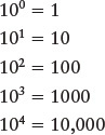
and so forth. Equivalently, the exponent tells you how many tens must be multiplied together to yield the desired number. For example, ten thousand can be written as 104 (“ten to the fourth”) because 104 = 10 × 10 × 10 × 10 = 10,000. Similarly, 273,000,000 can be written as 2.73 × 10⁸.
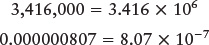
In scientific notation, numbers are written as a figure between 1 and 10 multiplied by the appropriate power of 10. The distance between Earth and the Sun, for example, can be written as 1.5 × 10⁸ km (or 9.3 × 10⁷ mi). Once you get used to it, you will find this notation more convenient than writing “150,000,000 kilometers” or “one hundred and fifty million kilometers.”
This powers-
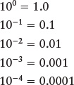
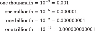
and so forth. For example, the diameter of a hydrogen atom is approximately 1.1 × 10⁻⁸ cm or (4.3 × 10⁻⁹ in). That is more convenient than saying “0.000000011 centimeter,” “11 billionths of a centimeter,” or the equivalent numbers in U.S. customary units. Similarly, 0.000728 equals 7.28 × 10⁻⁴.
Using the powers-
Because powers-
and also
Try these questions: Write 3,141,000,000 and 0.0000000031831 in scientific notation. Write 2.718282 × 10¹⁰ and 3.67879 × 10⁻¹¹ in standard notation.
(Answers appear at the end of the book.)
APPENDICES B-L
APPENDIX B: TEMPERATURE SCALES
Three temperature scales are in common use. Throughout most of the world, temperatures are expressed in degrees Celsius (°C), named in honor of the Swedish astronomer Anders Celsius, who proposed it in 1742. The Celsius temperature scale (also known as the “centigrade scale”) is based on the behavior of water, which freezes at 0°C and boils at 100°C at sea level on Earth.
Scientists usually prefer the Kelvin scale, named after the British physicist Lord Kelvin (William Thomson), who made many important contributions to our knowledge about heat and temperature. On the Kelvin temperature scale, water freezes at 273 K and boils at 373 K. Note that we do not use the degree symbol with the Kelvin temperature scale.
A-
Because water must be heated by 100 K or 100°C to go from its freezing point to its boiling point, you can see that the size of a kelvin is the same as the size of a degree Celsius. When considering temperature changes, measurements in kelvins and in degrees Celsius lead to the same number.
A temperature expressed in kelvins is always equal to the temperature in degrees Celsius plus 273. Scientists prefer the Kelvin scale because it is closely related to the physical meaning of temperature. All substances are made of atoms, which are very tiny (a typical atom has a diameter of about 10−10 m or 3.9 × 10⁻⁹ in) and constantly in motion. The temperature of a substance is directly related to the average speed of its atoms. If something is hot, its atoms are moving at high speeds. If a substance is cold, its atoms are moving much more slowly.
The coldest possible temperature is the temperature at which atoms move as slowly as possible (they can never quite stop completely). This minimum possible temperature, called absolute zero, is the starting point for the Kelvin scale. Absolute zero is 0 K, or −273°C. Because it is impossible for anything to be colder than 0 K, there are no negative temperatures on the Kelvin scale.
In the United States, many people still use the now outdated Fahrenheit scale, which expresses temperature in degrees Fahrenheit (°F). When the German physicist Gabriel Fahrenheit introduced this scale in the early 1700s, he intended 0°F to represent the coldest temperature then achievable (with a mixture of ice and saltwater) and 100°F to represent the temperature of a healthy human body. On the Fahrenheit scale, water freezes at 32°F and boils at 212°F. Because there are 180 degrees Fahrenheit between the freezing and boiling points of water, a degree Fahrenheit is only 100/180 (= 5/9) the size of the other scales.
The following equation converts from degrees Fahrenheit to degrees Celsius:
TC = 5/9 (TF − 32)
To convert from Celsius to Fahrenheit, a simple rearrangement of terms gives the relationship
TF = 9/5 TC + 32
where TF is the temperature in degrees Fahrenheit and TC is the temperature in degrees Celsius.
For example, consider a typical room temperature of 68°F. Using the first equation, we can convert this measurement to the Celsius scale as follows:
TC = 5/9 (68 − 32) = 20°C
To arrive at the Kelvin scale, we simply add 273 degrees to the value in degrees Celsius. Thus, 68°F = 20°C = 293 K. Figure B-
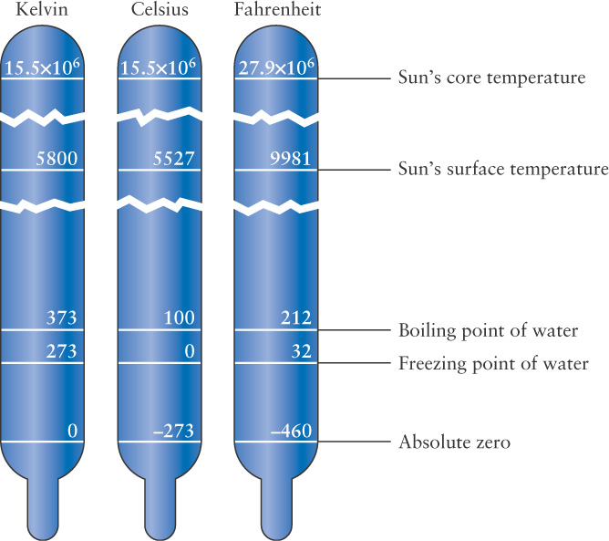
Try these questions: The Sun’s surface temperature is about 5800 K. What is its temperature in Celsius and Fahrenheit? The temperature of empty space is about 3 K. What is its temperature in Celsius and Fahrenheit? (Answers appear at the end of the book.)
A-
|
Planet |
Semimajor axis |
Sidereal period |
Synodic period (day) |
Mean orbital speed (km/s) |
Orbital eccentricity |
Inclination of orbit to ecliptic (°) |
||
|---|---|---|---|---|---|---|---|---|
|
(AU) |
(106 km) |
(year) |
(day) |
|||||
|
Mercury |
0.3871 |
57.9 |
0.2408 |
87.97 |
115.88 |
47.9 |
0.206 |
7.00 |
|
Venus |
0.7233 |
108.2 |
0.6152 |
224.70 |
583.92 |
35.0 |
0.007 |
3.39 |
|
Earth |
1.0000 |
149.6 |
1.0000 |
365.26 |
— |
29.8 |
0.017 |
0.00 |
|
Mars |
1.5237 |
227.9 |
1.8808 |
686.98 |
779.94 |
24.1 |
0.093 |
1.85 |
|
Jupiter |
5.2034 |
778.6 |
11.862 |
4,332.6 |
398.9 |
13.1 |
0.048 |
1.31 |
|
Saturn |
9.5371 |
1433.5 |
29.457 |
10,759 |
378.1 |
9.7 |
0.054 |
2.48 |
|
Uranus |
19.1913 |
2872.5 |
84.01 |
30,685 |
369.7 |
6.8 |
0.047 |
0.77 |
|
Neptune |
30.0690 |
4495.1 |
164.79 |
60,189 |
367.5 |
5.4 |
0.009 |
1.77 |
|
Planet |
Equatorial diameter |
Mass |
Mean density (kg/m3) |
Rotation period* (days) |
Inclination of equator to orbit (*) |
Surface gravity (Earth = 1) |
Albedo |
Escape speed (km/s) |
||
|---|---|---|---|---|---|---|---|---|---|---|
|
(km) |
(Earth = 1) |
(kg) |
(Earth = 1) |
|||||||
|
Mercury |
4,879 |
0.383 |
3.302 × 10²³ |
0.055 |
5427 |
58.646 |
173.4 |
0.38 |
0.106 |
4.3 |
|
Venus |
12,104 |
0.949 |
4.869 × 1024 |
0.815 |
5243 |
243.02R |
177.4 |
0.91 |
0.65 |
10.4 |
|
Earth |
12,756 |
1.000 |
5.974 × 1024 |
1.000 |
5515 |
0.996 |
23.45 |
1.000 |
0.37 |
11.2 |
|
Mars |
6,794 |
0.533 |
6.419 × 10²³ |
0.107 |
3933 |
1.025 |
25.19 |
0.38 |
0.15 |
5.0 |
|
Jupiter |
142,984 |
11.209 |
1.899 × 1027 |
317.83 |
1326 |
0.413 |
3.13 |
2.5 |
0.52 |
59.5 |
|
Saturn |
120,536 |
9.449 |
5.685 × 1026 |
95.16 |
687 |
0.445 |
26.73 |
1.1 |
0.47 |
35.5 |
|
Uranus |
51,118 |
4.007 |
8.683 × 1025 |
14.54 |
1270 |
0.717R |
97.77 |
0.91 |
0.51 |
21.3 |
|
Neptune |
49,528 |
3.883 |
1.024 × 1026 |
17.147 |
1638 |
0.671 |
28.32 |
1.1 |
0.4 |
23.5 |
* For Jupiter, Saturn, Uranus, and Neptune, the internal rotation period is given. A superscript R means that the rotation is retrograde (opposite the planet’s orbital motion).
A-
|
Planet |
Satellite |
Discoverers of moons |
Average distance from center of planet (km) |
Orbital (sidereal) period* (days) |
Orbital eccentricity |
Diameter of satellite (km) |
Mass (kg) |
|---|---|---|---|---|---|---|---|
|
EARTH |
Moon |
— |
384,400 |
27.322 |
0.0549 |
3476 |
7.349 × 10²² |
|
MARS |
Phobos |
Hall (1877) |
9,378 |
0.319 |
0.02 |
28 × 23 × 2 |
1.1 × 10¹⁶ |
|
|
Deimos |
Hall (1877) |
23,459 |
1.262 |
0.00 |
16 × 12 × 10 |
2.4 × 10¹⁵ |
|
JUPITER |
Io |
Galileo (1610) |
421,600 |
1.769 |
0.00 |
3643 |
8.93 × 10²² |
|
|
Europa |
Galileo (1610) |
670,900 |
3.551 |
0.01 |
3138 |
4.80 × 10²² |
|
|
Ganymede |
Galileo (1610) |
1,070,000 |
7.155 |
0.00 |
5268 |
1.48 × 10²³ |
|
|
Callisto |
Galileo (1610) |
1,883,000 |
16.689 |
0.01 |
4821 |
1.08 × 10²³ |
|
SATURN |
Mimas |
Herschel (1789) |
185,520 |
0.942 |
0.02 |
392 |
3.8 × 10¹⁹ |
|
|
Enceladus |
Herschel (1789) |
238,020 |
1.370 |
0.00 |
444 |
7.3 × 10¹⁹ |
|
|
Tethys |
Cassini (1684) |
294,660 |
1.888 |
0.00 |
1050 |
6.3 × 10²⁰ |
|
|
Dione |
Cassini (1684) |
377,400 |
2.737 |
0.00 |
1120 |
1.1 × 10²¹ |
|
|
Rhea |
Cassini (1672) |
527,040 |
4.518 |
0.00 |
1528 |
2.3 × 10²¹ |
|
|
Titan |
Huygens (1655) |
1,221,830 |
15.945 |
0.03 |
5150 |
1.3 × 10²³ |
|
|
Iapetus |
Cassini (1671) |
3,561,300 |
79.330 |
0.03 |
1436 |
1.6 × 10²¹ |
|
URANUS |
Miranda |
Kuiper (1948) |
129,872 |
1.413 |
0.00 |
−470 |
6.6 × 10¹⁹ |
|
|
Ariel |
Lassell (1851) |
190,945 |
2.520 |
0.00 |
−1160 |
1.4 × 10²¹ |
|
|
Umbriel |
Lassell (1851) |
265,998 |
4.144 |
0.01 |
1169 |
1.2 × 10²¹ |
|
|
Titania |
Herschel (1787) |
436,298 |
8.706 |
0.00 |
1578 |
3.5 × 10²¹ |
|
|
Oberon |
Herschel (1787) |
583,519 |
13.463 |
0.00 |
1523 |
3.0 × 10²¹ |
|
NEPTUNE |
Triton |
Lassell (1846) |
354,760 |
5.877R |
0.00 |
2704 |
2.14 × 10²² |
|
|
Nereid |
Kuiper (1949) |
5,513,400 |
360.1 |
0.75 |
340 |
2 × 10¹⁹ |
*A superscript R means that the satellite orbits in a retrograde direction (opposite to the planet’s rotation).
A-
|
Name* |
Parallax (arcsec) |
Distance (ly) |
Spectral type |
Radial velocity** (km/s) |
Proper motion (arcsec/year) |
Apparent visual magnitude |
Absolute visual magnitude |
Luminosity (Sun = 1) |
|---|---|---|---|---|---|---|---|---|
|
Sun |
|
|
G2 V |
|
|
−26.7 |
+4.85 |
1.00 |
|
Proxima Centauri |
0.769 |
4.22 |
M5.5 V |
−22 |
3.853 |
+11.09 |
+15.53 |
8.2 × 10⁻⁴ |
|
Alpha Centauri A |
0.747 |
4.40 |
G2 V |
−25 |
3.710 |
−0.01 |
+4.38 |
1.77 |
|
Alpha Centauri B |
0.747 |
4.40 |
K0 V |
−21 |
3.724 |
+1.34 |
+5.71 |
0.55 |
|
Barnard’s Star |
0.547 |
5.94 |
M4 V |
−111 |
10.358 |
+9.53 |
+13.22 |
3.6 × 10⁻³ |
|
Wolf 359 |
0.419 |
7.80 |
M6 V |
+13 |
4.696 |
+13.44 |
+16.6 |
3.5 × 10⁻⁴ |
|
Lalande 21185 |
0.393 |
8.32 |
M2 V |
−84 |
4.802 |
+7.47 |
+10.44 |
0.023 |
|
L 726- |
0.374 |
8.56 |
M5.5 V |
+29 |
3.368 |
+12.54 |
+15.4 |
9.4 × 10⁻⁴ |
|
L 726- |
0.374 |
8.56 |
M6 V |
+32 |
3.368 |
+12.99 |
+15.9 |
5.6 × 10⁻⁴ |
|
Sirius A |
0.380 |
8.61 |
A1 V |
−9 |
1.339 |
−1.43 |
+1.47 |
26.1 |
|
Sirius B |
0.380 |
8.61 |
white dwarf |
−9 |
1.339 |
+8.44 |
+11.34 |
2.4 × 10⁻³ |
|
Ross 154 |
0.337 |
9.71 |
M3.5 V |
−12 |
0.666 |
+10.43 |
+13.07 |
4.1 × 10⁻³ |
|
Ross 248 |
0.316 |
10.32 |
M5.5 V |
−78 |
1.617 |
+12.29 |
+14.8 |
1.5 × 10⁻³ |
|
Epsilon Eridani |
0.310 |
10.49 |
K2 V |
+17 |
0.977 |
+3.73 |
+6.19 |
0.40 |
|
Lacaille 9352 |
0.304 |
10.73 |
M1.5 V |
+10 |
6.896 |
+7.34 |
+9.75 |
0.051 |
|
Ross 128 |
0.299 |
10.87 |
M4 V |
−31 |
1.361 |
+11.13 |
+13.51 |
2.9 × 10⁻³ |
|
L 789- |
0.294 |
11.09 |
M5 V |
−60 |
3.259 |
+12.33 |
+14.7 |
1.3 × 10⁻³ |
|
61 Cygni A |
0.286 |
11.36 |
K5 V |
−65 |
5.281 |
+5.21 |
+7.49 |
0.16 |
|
61 Cygni B |
0.286 |
11.44 |
K7 V |
−64 |
5.172 |
+6.03 |
+8.31 |
0.095 |
|
Procyon A |
0.286 |
11.40 |
F5 IV– |
−4 |
1.259 |
+0.38 |
+2.66 |
7.73 |
|
Procyon B |
0.286 |
11.40 |
white dwarf |
−4 |
1.259 |
+10.7 |
+12.98 |
5.5 × 10⁻⁴ |
|
BD +59° 1915 A |
0.281 |
11.61 |
M3 V |
−1 |
2.238 |
+8.94 |
+11.18 |
0.020 |
|
BD +59° 1915 B |
0.281 |
11.61 |
M3.5 V |
+1 |
2.313 |
+9.70 |
+11.97 |
0.010 |
|
Groombridge 34 A |
0.281 |
11.65 |
M1.5 V |
+12 |
2.918 |
+8.08 |
+10.32 |
0.030 |
|
Groombridge 34 B |
0.281 |
11.65 |
M3.5 V |
+11 |
2.918 |
+11.06 |
+13.3 |
3.1 × 10⁻³ |
|
Epsilon Indi |
0.276 |
11.82 |
K5 V |
−40 |
4.704 |
+4.69 |
+6.89 |
0.27 |
|
GJ 1111 |
0.276 |
11.82 |
M6.5 V |
−5 |
1.290 |
+14.78 |
+16.98 |
2.7 × 10⁻⁴ |
|
Tau Ceti |
0.274 |
11.90 |
G8 V |
−17 |
1.922 |
+3.49 |
+5.68 |
0.62 |
|
GJ 1061 |
0.272 |
12.08 |
M5.5 V |
−20 |
0.826 |
+13.09 |
+15.26 |
1.0 × 10⁻³ |
|
L 725- |
0.269 |
12.12 |
M4.5 V |
+28 |
1.372 |
+12.10 |
+14.25 |
1.7 × 10⁻³ |
|
BD +05° 1668 |
0.263 |
12.40 |
M3.5 V |
+18 |
3.738 |
+9.84 |
+11.94 |
0.011 |
|
Kapteyn’s star |
0.255 |
12.79 |
M1.5 V |
+246 |
8.670 |
+8.84 |
+10.87 |
0.013 |
|
Lacaille 8760 |
0.253 |
12.89 |
M0 V |
+28 |
3.455 |
+6.67 |
+8.69 |
0.094 |
|
Krüger 60 A |
0.248 |
13.05 |
M3 V |
−33 |
0.990 |
+9.79 |
+11.76 |
0.010 |
|
Krüger 60 B |
0.248 |
13.05 |
M4 V |
−32 |
0.990 |
+11.41 |
+13.38 |
3.4 × 10⁻³ |
*Stars that are components of binary systems are labeled A and B.
**A positive radial velocity means the star is receding; a negative radial velocity means the star is approaching.
Compiled from the Hipparcos General Catalogue and from data reported by the Research Consortium on Nearby Stars. The table lists all known stars within 4.00 parsecs (13.05 light-
A-
|
Name |
Designation |
Distance (ly) |
Spectral type |
Radial velocity* (km/s) |
Proper motion (arcsec/year) |
Apparent visual magnitude |
Apparent visual brightness** (Sirius = 1) |
Absolute visual magnitude |
Luminosity (Sun = 1) |
|---|---|---|---|---|---|---|---|---|---|
|
Sirius A |
α CMa A |
8.61 |
A1 V |
−9 |
1.339 |
−1.43 |
1.000 |
+1.47 |
26.1 |
|
Canopus |
α Car |
313 |
F0 I |
+21 |
0.031 |
−0.62 |
0.470 |
−5.53 |
1.4 × 10⁴ |
|
Arcturus |
α Boo |
36.7 |
K2 III |
−5 |
2.279 |
−0.05 |
0.278 |
−0.31 |
190 |
|
Rigil Kentaurus |
α Cen A |
4.4 |
G2 V |
−25 |
3.71 |
−0.01 |
0.268 |
+4.38 |
1.77 |
|
Vega |
α Lyr |
25.3 |
A0 V |
−14 |
0.035 |
+0.03 |
0.258 |
+0.58 |
61.9 |
|
Capella |
α Aur |
42.2 |
G8 III |
+30 |
0.434 |
+0.08 |
0.247 |
−0.48 |
180 |
|
Rigel |
β Ori A |
773 |
B8 Ia |
+21 |
0.002 |
+0.18 |
0.225 |
−6.69 |
7.0 × 10⁵ |
|
Procyon |
α CMi A |
11.4 |
F5 IV- |
−4 |
1.259 |
+0.38 |
0.184 |
+2.66 |
7.73 |
|
Achernar |
α Eri |
144 |
B3 IV |
+19 |
0.097 |
+0.45 |
0.175 |
−2.77 |
5250 |
|
Betelgeuse |
α Ori |
427 |
M2 Iab |
+21 |
0.029 |
+0.45 |
0.175 |
−5.14 |
4.1 × 10⁴ |
|
Hadar |
β Cen |
525 |
B1 II |
−12 |
0.042 |
+0.61 |
0.151 |
−5.42 |
8.6 × 10⁴ |
|
Altair |
α Aql |
16.8 |
A7 IV- |
−26 |
0.661 |
+0.77 |
0.132 |
+2.2 |
11.8 |
|
Aldebaran |
α Tau A |
65.1 |
K5 III |
+54 |
0.199 |
+0.87 |
0.119 |
−0.63 |
370 |
|
Spica |
α Vir |
262 |
B1 V |
+1 |
0.053 |
+0.98 |
0.108 |
−3.55 |
2.5 × 10⁴ |
|
Antares |
α Sco A |
604 |
M1 Ib |
−3 |
0.025 |
+1.06 |
0.100 |
−5.28 |
3.7 × 10⁴ |
|
Pollux |
β Gem |
33.7 |
K0 III |
+3 |
0.627 |
+1.16 |
0.091 |
+1.09 |
46.6 |
|
Fomalhaut |
α PsA |
25.1 |
A3 V |
+7 |
0.368 |
+1.17 |
0.090 |
+1.74 |
18.9 |
|
Deneb |
α Cyg |
3230 |
A2 Ia |
−5 |
0.002 |
+1.25 |
0.084 |
−8.73 |
3.2 × 10⁵ |
|
Mimosa |
β Cru |
353 |
B0.5 III |
+20 |
0.05 |
+1.25 |
0.084 |
−3.92 |
3.4 × 10⁴ |
|
Regulus |
α Leo A |
77.5 |
B7 V |
+4 |
0.249 |
+1.36 |
0.076 |
−0.52 |
331 |
Data in this table compiled from the Hipparcos General Catalogue.
*A positive radial velocity means the star is receding; a negative radial velocity means the star is approaching.
**This is the ratio of the star’s apparent brightness to that of Sirius, the brightest star in the night sky.
Note: Acrux, or α Cru (the brightest star in Crux, the Southern Cross), appears to the naked eye as a star of apparent magnitude +0.87, the same as Aldebaran, but it does not appear in this table because Acrux is actually a binary star system. The blue-
A-
|
Name |
Meaning |
R.A. |
Dec. |
Genitive* |
Abbreviation |
|---|---|---|---|---|---|
|
Andromeda |
proper name; princess |
1 |
+40 |
Andromedae |
And |
|
Antlia |
air pump |
10 |
−35 |
Antliae |
Ant |
|
Apus |
bee |
16 |
−75 |
Apodis |
Aps |
|
Aquarius1,2 |
waterman |
22 |
−10 |
Aquarii |
Aqr |
|
Aquila |
eagle |
20 |
+15 |
Aquilae |
Aql |
|
Ara |
altar |
17 |
−55 |
Arae |
Ara |
|
Aries2 |
ram |
3 |
+20 |
Arietis |
Ari |
|
Auriga |
charioteer |
6 |
+40 |
Aurigae |
Aur |
|
Boötes |
proper name; herdsman, wagoner |
15 |
+30 |
Boötis |
Boo |
|
Caelum |
engraving tool |
5 |
−40 |
Caeli |
Cae |
|
Camelopardalis |
giraffe |
6 |
+70 |
Camelopardalis |
Cam |
|
Cancer2 |
crab |
8.5 |
+15 |
Cancri |
Cnc |
|
Canes Venatici |
hunting dogs |
13 |
+40 |
Canum Venaticorum |
CVn |
|
Canis Major |
larger dog |
7 |
−20 |
Canis Majoris |
CMa |
|
Canis Minor |
smaller dog |
8 |
+5 |
Canis Minoris |
CMi |
|
Capricornus1,2 |
water– |
21 |
−20 |
Capricornii |
Cap |
|
Carina |
keel |
9 |
−60 |
Carinae |
Car |
|
Cassiopeia |
proper name; queen |
1 |
+60 |
Cassiopeiae |
Cas |
|
Centaurus |
centaur |
13 |
−45 |
Centauri |
Cen |
|
Cepheus |
proper name; king |
22 |
+65 |
Cephei |
Cep |
|
Cetus |
whale |
2 |
−10 |
Ceti |
Cet |
|
Chamaeleon |
chameleon |
10 |
−80 |
Chamaeleontis |
Cha |
|
Circinus |
compasses |
15 |
−65 |
Circini |
Cir |
|
Columba |
dove |
6 |
−35 |
Columbae |
Col |
|
Coma Berenices |
Berenice’s hair |
13 |
+20 |
Comae Berenices |
Com |
|
Corona Australis3 |
southern crown |
19 |
+40 |
Coronae Australis |
CrA |
|
Corona Borealis4 |
northern crown |
16 |
+30 |
Coronae Borealis |
CrB |
|
Corvus5 |
crow, raven |
12 |
−20 |
Corvi |
Crv |
|
Crater |
cup |
11 |
−15 |
Crateris |
Crt |
|
Crux6 |
southern cross |
12 |
−60 |
Crucis |
Cru |
|
Cygnus |
swan |
21 |
+40 |
Cygni |
Cyg |
|
Delphinus1 |
dolphin |
21 |
+10 |
Delphini |
Del |
|
Dorado7 |
swordfish |
6 |
−55 |
Doradus |
Dor |
|
Draco8 |
dragon |
15 |
+60 |
Draconis |
Dra |
|
Equuleus |
little horse |
21 |
+10 |
Equulei |
Equ |
|
Eridanus |
proper name; river |
4 |
−30 |
Eridani |
Eri |
|
Fornax |
furnace |
3 |
−30 |
Fornacis |
For |
|
Gemini2 |
twins |
7 |
+20 |
Geminorum |
Gem |
|
Grus |
crane |
22 |
−45 |
Gruis |
Gru |
|
Hercules9 |
proper name; hero |
17 |
+30 |
Herculis |
Her |
|
Horologium |
clock |
3 |
−55 |
Horologii |
Hor |
|
Hydra |
water serpent |
12 |
−25 |
Hydrae |
Hya |
|
Hydrus |
water snake |
2 |
−70 |
Hydri |
Hyi |
|
Indus |
Indian |
22 |
−70 |
Indi |
Ind |
|
Lacerta |
lizard |
22 |
+45 |
Lacertae |
Lac |
|
Leo2 |
lion |
11 |
+15 |
Leonis |
Leo |
|
Leo Minor |
smaller lion |
10 |
+35 |
Leonis Minoris |
LMi |
|
Lepus |
hare |
6 |
−20 |
Leporis |
Lep |
|
Libra2,10 |
scales |
15 |
−15 |
Librae |
Lib |
|
Lupus |
wolf |
15 |
−45 |
Lupi |
Lup |
|
Lynx |
lynx |
8 |
+45 |
Lyncis |
Lyn |
|
Lyra5 |
lyre |
19 |
+35 |
Lyrae |
Lyr |
|
Microscopium |
microscope |
21 |
−40 |
Microscopii |
Mic |
|
Monoceros |
unicorn |
7 |
0 |
Monocerotis |
Mon |
|
Mensa |
table |
6 |
−75 |
Mensae |
Men |
|
Musca (Australis)11 |
(southern) fly |
12 |
−70 |
Muscae |
Mus |
|
Norma |
square |
16 |
−50 |
Normae |
Nor |
|
Octans12 |
octant |
— |
−90 |
Octantis |
Oct |
|
Ophiuchus2,13 |
serpent- |
17 |
0 |
Ophiuchi |
Oph |
|
Orion |
proper name; hunter, giant |
6 |
0 |
Orionis |
Ori |
|
Pavo |
peacock |
20 |
−70 |
Pavonis |
Pav |
|
Pegasus |
proper name; winged horse |
23 |
+20 |
Pegasi |
Peg |
|
Perseus |
proper name; hero |
3 |
+45 |
Persei |
Per |
|
Phoenix |
phoenix |
1 |
−50 |
Phoenicis |
Phe |
|
Pictor |
easel |
6 |
−55 |
Pictoris |
Pic |
|
Pisces1,2 |
fishes |
1 |
+10 |
Piscium |
Psc |
|
Piscis Austrinus1 |
southern fish |
22 |
−30 |
Piscis Austrini |
PsA |
|
Puppis |
stern |
8 |
−30 |
Puppis |
Pup |
|
Pyxis |
compass |
9 |
−30 |
Pyxidis |
Pyx |
|
Reticulum |
net |
4 |
−60 |
Reticuli |
Ret |
|
Sagitta |
arrow |
20 |
+20 |
Sagittae |
Sge |
|
Sagittarius2,14 |
archer |
19 |
−25 |
Sagittarii |
Sgr |
|
Scorpius2 |
scorpion |
17 |
−30 |
Scorpii |
Sco |
|
Sculptor15 |
sculptor’s workshop |
1 |
−30 |
Sculptoris |
Scl |
|
Scutum16 |
shield |
19 |
−10 |
Scuti |
Sct |
|
Sextans |
sextant |
10 |
0 |
Sextantis |
Sex |
|
Taurus2 |
bull |
5 |
+20 |
Tauri |
Tau |
|
Telescopium |
telescope |
19 |
−50 |
Telescopii |
Tel |
|
Triangulum |
triangle |
2 |
+30 |
Trianguli |
Tri |
|
Triangulum Australe |
southern triangle |
16 |
−65 |
Trianguli Australis |
TrA |
|
Tucana17 |
toucan |
0 |
−65 |
Tucanae |
Tuc |
|
Ursa Major |
larger bear |
11 |
+60 |
Ursae Majoris |
UMa |
|
Ursa Minor18 |
smaller bear |
16 |
+80 |
Ursae Minoris |
UMi |
|
Vela |
sails |
10 |
−45 |
Velorum |
Vel |
|
Virgo2 |
virgin |
13 |
0 |
Virginis |
Vir |
|
Volans |
flying fish |
8 |
−70 |
Volantis |
Vol |
|
Vulpecula |
fox |
20 |
+25 |
Vulpeculae |
Vul |
*Genitive is the grammatical case denoting possession. For example, astronomers denote the brightest or α (alpha) star in Orion (Betelgeuse) as α Orionis.
1Constellations of the area of the sky known as the wet quarter for its many watery images.
2A zodiac constellation.
3Sometimes considered as Sagittarius’s crown.
4Ariadne’s crown.
5Corvus was Orpheus’s companion, Lyra his harp.
6Originally a part of Centaurus.
7Contains the Large Magellanic Cloud and the south ecliptic pole.
8Contains the north ecliptic pole.
9One of the oldest constellations known.
10Originally the claws of Scorpius.
11Originally named Musca Australis to distinguish it from Musca Borealis, the northern fly, which is now defunct; “Australis” is now dropped.
12Contains the south celestial pole.
13Ophiucus is identified with the physician Aesculapius, and Serpens with the caduceus.
14Contains the galactic center.
15Originally named by Lacaille l’Atelier du Sculpteur (in Latin, Apparatus Sculptoris); now known simply as Sculptor. Contains the south galactic pole.
16Shield of the Polish hero John Sobieski.
17Contains the Small Magellanic Cloud.
18Contains the north celestial pole.
A-
A-
A-
|
Astronomical unit: |
1 AU = 1.496 × 10¹¹ m |
|
Light- |
1 ly = 9.461 × 10¹⁵ m = 63,240 AU |
|
Parsec: |
1 pc = 3.086 × 10¹⁶ m = 3.262 ly |
|
Solar mass: |
1 M⊙ = 1.989 × 1030 kg |
|
Solar radius: |
1 R⊙ = 6.960 × 10⁸ m |
|
Solar luminosity: |
1 L⊙ = 3.827 × 1026 W |
|
Earth’s mass: |
1 M⊕ = 5.974 × 1024 kg |
|
Earth’s equatorial radius: |
1 R⊕ = 6.378 × 10⁶ m |
|
Moon’s mass: |
1 MMoon = 7.349 × 10²² kg |
|
Moon’s equatorial radius: |
1 RMoon = 1.738 × 10⁶ m |
|
Speed of light: |
c = 2.998 × 10⁸ m/s |
|
Gravitational constant: |
G = 6.668 × 10⁻¹¹ N m2 kg−2 |
|
Planck constant: |
h = 6.626 × 10⁻³⁴ J s = 4.136 × 10⁻¹⁵ eV s |
|
Boltzmann constant: |
k = 1.380 × 10⁻²³ J K−1 = 8.617 × 10⁻⁵ eV K−1 |
|
Stefan– |
σ = 5.670 × 10⁻⁸ W m−2 K−4 |
|
Mass of electron: |
me = 9.109 × 10⁻³¹ kg |
|
Mass of 1 H atom: |
mH = 1.673 × 10⁻²⁷ kg |
|
1 inch = 2.54 centimeters (cm) |
|
1 cm = 0.394 inch (in) |
|
1 yard = 0.914 meter (m) |
|
1 meter = 1.09 yards = 39.37 inches |
|
1 mile = 1.61 kilometers (km) |
|
1 km = 0.621 mile (mi) |
A-
|
|
Individual contribution |
Section total |
|---|---|---|
|
Dark matter and dark energy contributions |
|
0.954 ± 0.003* |
|
Dark energy |
0.72 ± 0.03 |
|
|
Dark matter |
0.23 ± 0.03 |
|
|
Primeval gravitational radiation |
≤10−10 |
|
|
Contributions from Big Bang era |
|
0.0010 ± 0.0005 |
|
Electromagnetic radiation |
10−4.3 ± 0.000001 |
|
|
Neutrinos |
10−2.9 ± 0.1 |
|
|
Normal particle (baryon) rest mass |
|
0.045 ± 0.003 |
|
Charged particles (plasma) between stars and galaxies |
0.0418 ± 0.003 |
|
|
Main- |
0.0015 ± 0.0004 |
|
|
Neutral hydrogen and helium |
0.00062 ± 0.00010 |
|
|
Main- |
0.00055 ± 0.00014 |
|
|
White dwarfs |
0.00036 ± 0.00008 |
|
|
Molecular gas |
0.00016 ± 0.00006 |
|
|
Substellar objects |
0.00014 ± 0.00007 |
|
|
Black holes |
0.00007 ± 0.00002 |
|
|
Neutron stars |
0.00005 ± 0.00002 |
|
|
Planets |
10−6 ± 0.1 |
|
*The numbers after the plus or minus (±) symbol indicate the possible errors in the given numbers.
This table lists the major contributions to the mass and energy of the universe.
APPENDIX M: READING GRAPHS
Reading Graphs
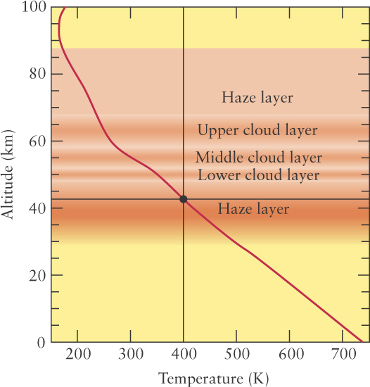
The graphs you will encounter in this book are compact ways of displaying patterns of information relating two variables, like the temperature and luminosity of stars or the temperature of an atmosphere at different altitudes. The relevant values of one of the variables are presented along the horizontal or x axis, and the relevant values of the other variable are presented along the vertical or y axis. The word “relevant” here indicates that often graphs do not start at 0. Consider three examples. First is data presented in Chapter 6 concerning the temperature of Venus’s atmosphere at different altitudes (Figure M-
A-
The horizontal axis of the graph indicates the temperature in kelvins (K). (Unlike degrees Celsius or degrees Fahrenheit, temperature using the Kelvin scale is simply noted as kelvins.)
The vertical axis denotes the altitude above Venus’s surface in kilometers (km). Note that both axes are always labeled with a name (temperature or altitude, here) and units (K or km, respectively). Bear in mind that some variables in graphs you will see in this book increase to the right or upward (these are more common), but some variables will increase in the opposite directions. To read a graph, note that a value on the horizontal axis is transferred directly upward through the graph. For example, all points on the blue line in Figure M-
A curve or a set of points on the graph presents the relationship between the variable represented on the horizontal axis and the variable on the vertical axis. Each point on a curve or each separate point relates the two variables. Choose a point, say, the dot on Figure M-
The red curve in Figure M-
Try these questions: What is the temperature at 20 km? What is the altitude at which the temperature is 300 K? For most of this graph, what is the general trend of the temperature with height? (Answers appear at the end of the book.)
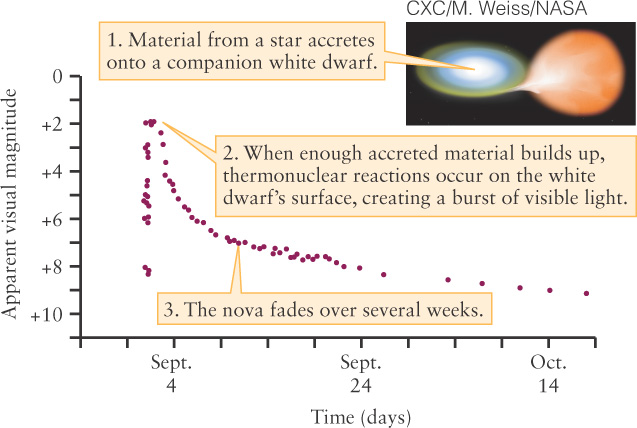
Sometimes, the known information is not a curve, but rather a set of points, as in our second example (Figure M-
Try these questions: What is the apparent magnitude on September 24? October 9? On what two days was the apparent magnitude +6? (Answers appear at the end of the book.)
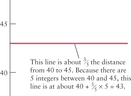
The graphs so far have shown variables that change uniformly along the axes. For example, the distance on Figure M-
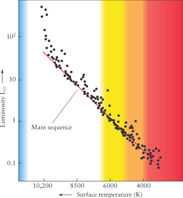
A-
The purpose of logarithmic and other nonlinear axes is to present in compact form data that vary very widely in values. For example, the dimmest star represented in Figure M-
Referring to Figure M-
Try these questions: Approximately what is the luminosity of a star with surface temperature 8500 K? What is the surface temperature of a star with the same luminosity as the Sun (1 L⊙)?
(Answers appear at the end of the book.)
A-
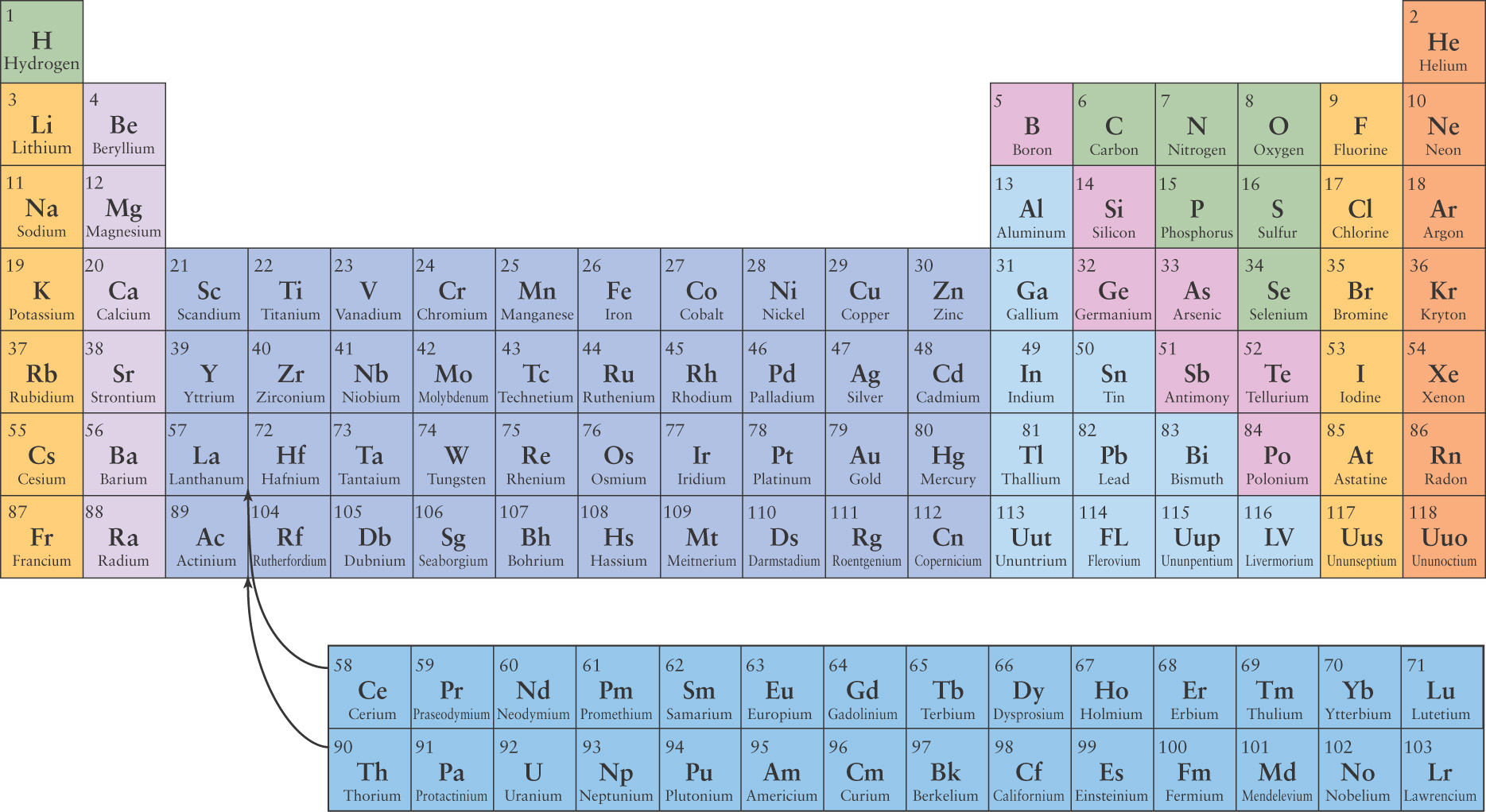
APPENDIX N: PERIODIC TABLE OF THE ELEMENTS
A-
APPENDIX O: TIDES
Tides result from a combination of Earth’s motion around its barycenter with the Moon (or Sun) and the changing strength of the gravitational force from the Moon (or Sun) across Earth. Ignoring Earth’s rotation and focusing on the Moon for the moment, let’s first consider the motion of Earth and the Moon around their barycenter (see Figure 6-
Opposing this force away from the Moon, Earth also has a gravitational attraction to its satellite. Recall from Section 2-
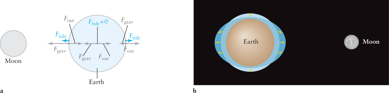
Because forces in the same or opposite directions simply add or subtract, respectively, we can subtract the two forces Fout and Fgrav at any point on Earth, due to the presence of the Moon. The resulting net force is labeled Ftide in Figure O-
Consider the point on Earth closest to the Moon. The strength of the tidal force, Ftide, seems to imply that the Moon’s gravitational force lifts the water there to create the high tide. However, the force of gravitation from the Moon is not strong enough to raise that water more than a few centimeters or inches. Rather, the high tide closest to the Moon occurs because ocean waters from nearly halfway around to the opposite side of Earth are pulled Moonward by the gravitational force acting on them. This water slides toward the Moon and fills the ocean directly under it, creating a tidal bulge or high tide. Likewise, the net outward force acting on the opposite side of Earth from the Moon pushes the waters that are just over halfway around from the Moon to the side directly away from it, creating a simultaneous second high tide of equal magnitude on the opposite side of Earth from the Moon. Where the water has been drained away in this process, low tides occur.
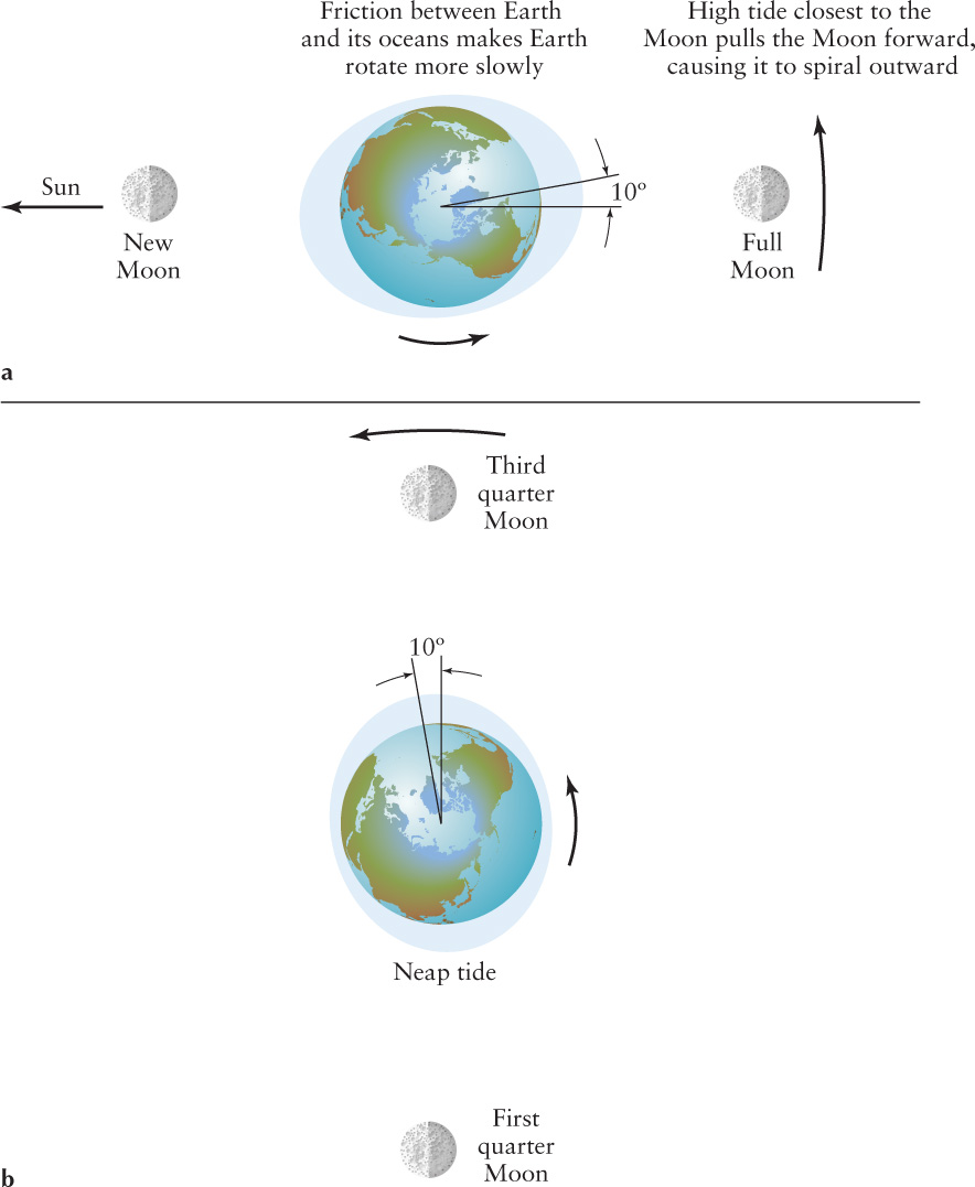
Let’s spin Earth back up. As it rotates, the geographic locations of the high and low tides continually change. Figure O-
Tides are complicated by the fact that the oceans are not uniformly deep, and the shores around continents and islands have a variety of shapes. As a result, in some places the oceans have only a single cycle of tides each day. Some places have tides that change negligibly, while some channels, such as the Bay of Fundy between the United States and Canada (maximum range between high and low tides of 16.3 m or 17.8 yd) and the Bristol Channel between Wales and England (maximum range of 15 m or 16.4 yd), have two tides that are each much higher than normal.
A-
Earth’s rotation also has the effect of moving the high tides away from the line between the centers of Earth and the Moon. Earth’s eastward rotation is nearly 30 times faster than the Moon’s eastward revolution around Earth. Therefore, as it rotates, Earth drags the high tides eastward with it. As a result, the high tide that should be directly between the centers of Earth and the Moon is actually 10° ahead of the Moon in its orbit around Earth (Figure O-
We can repeat this analysis for the Earth–
APPENDIX P: ENERGY AND MOMENTUM
Scientists identify two types of energy that are available to any object. The first, called kinetic energy, is associated with the object’s motion. For speeds much less than the speed of light, we can write the amount of kinetic energy, KE, of an object as

where m is the object’s mass and v is its speed. Kinetic energy is a measure of how much work the object can do on the outside world or, equivalently, how much work the outside world has done to give the object this speed. Kinetic energy applies to rotation and revolution, as well as to straight-
Work is also a rigorously defined concept that often is at odds with our intuition. Work is defined as the product of the force, F, acting on an object and the distance, d, over which the object moves in the direction of the force:
W = Fd
For example, if I exert a horizontal force of 50 N (N is the unit newtons and is the metric unit of force) and thereby move an object 10 m in the direction I push it, then I have done 50 N × 10 m = 500 J of work. (I have used the relationship that 1 newton × 1 meter = 1 joule.)
The second type of energy is called potential energy, the energy available to an object as a result of its location in space. For example, if you hold a pencil above the ground, the pencil has potential energy that can be converted into kinetic energy by Earth’s gravitational force. How does that conversion get underway? Just let go of the pencil.
There are various kinds of potential energy, such as the potential energy stored in a battery and the potential energy stored in objects under the influence of gravity. We will focus on gravitational potential energy. Far from extremely massive objects, like stars, or extremely dense objects, like black holes, gravitational potential energy, PE, can be written as

where the constant G = 6.6683 × 10⁻¹¹ N m2/kg2, m is the mass of the object whose gravitational potential energy you are measuring, M is the mass of the object generating the gravitational attraction, and r is the distance between the centers of mass of these two objects.
Near the surface of Earth, this equation simplifies to
PE = mgh
A-
where g = 9.8 m/s2 (32 ft/s2) is the gravitational acceleration at Earth’s surface, and h is the height of the object above Earth’s surface.
Potential energy can be converted into kinetic energy and vice versa. After you drop a pencil, its gravitational potential energy begins to decrease while its kinetic energy begins to increase at the same rate. The pencil’s total energy is conserved. Conversely, if you throw a pencil up in the air, the kinetic energy you give it will immediately begin to decrease, while its potential energy increases at the same rate.
Related to the motion of an object and, hence, to its kinetic energy are the concepts of linear momentum, usually just called momentum, and angular momentum. Momentum, p, is described by the equation
p = mv
where v is the velocity of the object. Both p and v are in boldface to indicate that they both represent motion in some direction or another (both in the same direction), as well as a numeric value. Simple algebra reveals that kinetic energy and momentum are related by

Linear momentum, then, indicates how much energy is available to an object because of its motion in a straight line (linear motion).
Angular momentum, L, can be expressed mathematically as
L = Iω
where I is the moment of inertia of an object, and ω (lowercase Greek omega) is the angular speed and direction of the rotating object. Just as an object’s mass indicates how hard it is to change an object’s straight-

Newton’s first law can also be expressed in terms of conservation of linear momentum:
A body maintains its linear momentum unless acted upon by a net external force.
Equivalently, for angular motion we can write the conservation of angular momentum:
A body maintains its angular momentum unless acted upon by a net external torque.
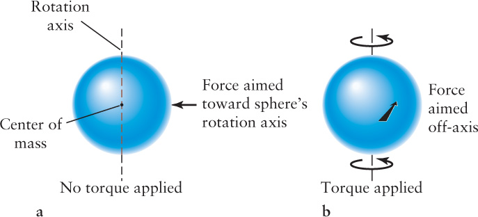
Torques are created when a force acts on an object in some direction other than toward the center of the object’s angular motion, as shown in Figure P-
Earth has angular momentum from two sources, namely, from spinning on its rotation axis and from orbiting the Sun. Likewise, the Moon has angular momentum because it spins on its rotation axis and it orbits Earth. Virtually all objects in astronomy have angular momentum, and it is probably fair to say that conservation of angular momentum is among the most important laws in the cosmos. After all, conservation of angular momentum is what keeps the planets in orbit around the Sun, the moons in orbit around the planets, and astronomical bodies rotating at relatively constant rates, as well as causing many other rotation-
Try these questions: How does tripling the linear momentum of an object change its kinetic energy? How does halving the angular momentum of an object change its kinetic energy? How much work would you do if you pushed on a desk with a force of 100 N, while it moved 20 m? How much work would you do if you pushed on a desk with a force of 500 N, and it moved 0 m? What two things can you vary to change the angular momentum of an object?
(Answers appear at the end of the book.)
A-
APPENDIX Q: RADIOACTIVITY AND THE AGES OF OBJECTS
The isotopes of many elements are radioactive, meaning that the elements spontaneously transform into other elements. Each radioactive isotope has a distinctive half-
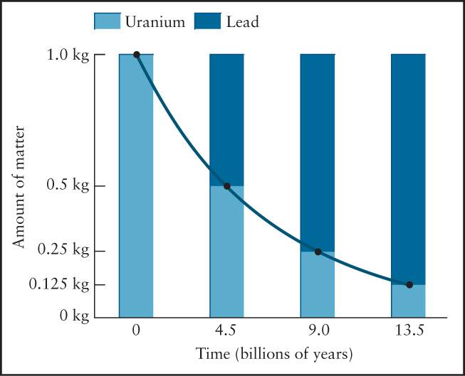
To determine the time since an object, such as a piece of space debris discovered on Earth, solidified, scientists estimate how much lead the object had when it formed. Then they measure the amounts of uranium and lead that it contains now. Subtracting the amount of original lead, they use the amount of uranium and lead, together with the graph of radioactive decay, to determine the object’s age.
Example: Suppose a piece of space debris discovered on Earth was determined to have equal amounts of lead and uranium. How long ago did this debris form? Assuming that it originally had no lead, we see from the chart that a 1-
Compare! This process works with any radioactive isotope. However, some isotopes have such short half-
Try these questions: What fraction of a kilogram of radioactive material remains after three half-
(Answers appear at the end of the book.)
APPENDIX R: GRAVITATIONAL FORCE
From Newton’s law of gravitation, if two objects that have masses m1 and m2 are separated by a distance r, then the gravitational force, F, between them is

In this formula, G is the universal constant of gravitation.
The equation F = G(m1m2/r2) gives, for example, the force from the Sun on Earth and, equivalently, the force from Earth on the Sun. If m1 is the mass of Earth (6.0 × 1024 kg), m2 is the mass of the Sun (2.0 × 1030 kg), and r is the distance from the center of Earth to the center of the Sun (1.5 × 10¹¹ m):
F = 3.6 × 10²² N
where N is the unit of force, a newton. This number can then be used in Newton’s second law, F = ma, to find the acceleration of Earth due to the Sun. This yields
aEarth = F/mEarth = 6.0 × 10⁻² m/s2
Newton’s third law says that Earth exerts the same force on the Sun, so the Sun’s acceleration due to Earth’s gravitational force is
aSun = F/mSun = 1.8 × 10⁻⁸ m/s2
In other words, Earth pulls on the Sun, causing the Sun to move toward it. Because of the Sun’s greater mass, however, the amount that the Sun accelerates Earth is more than 300,000 times greater than the amount that Earth accelerates the Sun.
Try these questions: Earth’s radius is 6.4 × 10⁶ m and 1 kg is a mass equivalent to a weight of 9.8 N (or 2.2 lb) on Earth. What is the force that Earth exerts on you in newtons and pounds? What is the force that you exert on Earth in these units? What would the Sun’s force (in newtons) be on Earth if our planet were twice as far from the Sun as it is? How does that force compare to the force from the Sun at our present location? (Answers appear at the end of the book.)
APPENDIX S: LARGEST OPTICAL TELESCOPES IN THE WORLD
A-
|
Aperture (m) |
Name |
Location |
Altitude (m) |
|---|---|---|---|
|
10.4 |
Gran Telescopio Cararias |
La Palma, Canary Islands, Spain |
2400 |
|
10 |
Keck I |
Mauna Kea, Hawaii |
4123 |
|
10 |
Keck II |
Mauna Kea, Hawaii |
4123 |
|
10 |
SALT |
Sutherland, South Africa |
1759 |
|
9.2 |
Hobby- |
Mt. Fowlkes, Texas |
2072 |
|
8.4 × 2 |
Large Binocular Telescope |
Mt. Graham, Arizona |
3170 |
|
8.3 |
Subaru |
Mauna Kea, Hawaii |
4100 |
|
8.2 |
Antu |
Cerro Paranal, Chile |
2635 |
|
8.2 |
Kueyen |
Cerro Paranal, Chile |
2635 |
|
8.2 |
Melipal |
Cerro Paranal, Chile |
2635 |
|
8.2 |
Tepun |
Cerro Paranal, Chile |
2635 |
|
8.1 |
Gemini North (Gillett) |
Mauna Kea, Hawaii |
4100 |
|
8.1 |
Gemini South |
Cerro Pachon, Chile |
2737 |
|
6.5 |
MMT |
Mt. Hopkins, Arizona |
2600 |
|
6.5 |
Walter Baade |
La Serena, Chile |
2282 |
|
6.5 |
Landon Clay |
La Serena, Chile |
2282 |
|
6 |
Bolshoi Teleskop Azimutalnyi |
Nizhny Arkhyz, Russia |
2070 |
|
6 |
LZT |
British Columbia, Canada |
395 |
|
5 |
Hale |
Palomar Mtn., California |
1900 |
|
4.2 |
William Herschel |
La Palma, Canary Islands, Spain |
2400 |
|
4.2 |
SOAR |
Cerro Pachon, Chile |
2738 |
|
4.2 |
LAMOST |
Xinglong Station, China |
950 |
|
4 |
Victor Blanco |
Cerro Tololo, Chile |
2200 |
|
3.9 |
Anglo- |
Coonabarabran, Australia |
1100 |
|
3.8 |
Mayall |
Kitt Peak, Arizona |
2100 |
|
3.8 |
UKIRT |
Mauna Kea, Hawaii |
4200 |
|
3.7 |
AEOS |
Maui, Hawaii |
3058 |
|
3.6 |
“360” |
Cerro La Silla, Chile |
2400 |
|
3.6 |
Canada- |
Mauna Kea, Hawaii |
4200 |
|
3.6 |
Telescopio Nazionale Galileo |
La Palma, Canary Islands, Spain |
2387 |
|
3.5 |
MPI- |
Calar Alto, Spain |
2200 |
|
3.5 |
New Techonology |
Cerro La Silla, Chile |
2400 |
|
3.5 |
ARC |
Apache Point, New Mexico |
2788 |
|
3.5 |
WIYN |
Kitt Peak, Arizona |
2100 |
|
3.5 |
Starfire |
Kirtland Air Force Base, New Mexico |
1900 |
|
3 |
Shane |
Mt. Hamilton, California |
1300 |
|
3 |
NASA IRTF |
Mauna Kea, Hawaii |
4160 |
|
2.7 |
Harlan Smith |
Mt. Locke, Texas |
2100 |
|
2.6 |
BAO |
Byurakan, Armenia |
1405 |
|
2.6 |
Shajn |
Crimea, Ukraine |
600 |
|
2.5 |
Hooker |
Mt. Wilson, California |
1700 |
|
2.5 |
Isaac Newton |
La Palma, Canary Islands, Spain |
2382 |
|
2.5 |
Nordic Optical |
La Palma, Canary Islands, Spain |
2382 |
|
2.5 |
duPont |
La Serena, Chile |
2282 |
|
2.5 |
Sloan Digital Sky Survey |
Apache Point, New Mexico |
2788 |
|
2.4 |
Hiltner |
Kitt Peak, Arizona |
2100 |
|
2.4 |
Lijiang |
Lijiang City, China |
3250 |
|
2.4 |
Hubble Space Telescope |
Low Earth orbit |
6 × 10⁵ |
|
2.3 |
WIRO |
Jelm Mtn., Wyoming |
2900 |
|
2.3 |
ANU |
Coonabarabran, Australia |
1100 |
|
2.3 |
Bok |
Kitt Peak, Arizona |
2100 |
|
2.3 |
Vainu Bappu |
Kavalur, India |
700 |
|
2.3 |
Aristarchos |
Mt. Helmos, Greece |
2340 |
|
2.2 |
ESO- |
Cerro La Silla, Chile |
2335 |
|
2.2 |
MPI- |
Calar Alto, Spain |
2200 |
|
2.2 |
UH |
Mauna Kea, Hawaii |
4200 |
|
2.1 |
Kitt Peak 2.1 meter |
Kitt Peak, Arizona |
2100 |
|
2.1 |
Otto Struve |
Davis Mountains, Texas |
2070 |
|
2.1 |
UNAM |
San Pedro, Mexico |
2800 |
|
2.1 |
Jorge Sahade |
El Leoncito, Argentina |
2552 |
|
2 |
Himalayan Chandra |
Hanle, India |
4517 |
|
2 |
Alfred Jensch Teleskop |
Tautenburg, Germany |
|
|
2 |
Carl Zeiss Jena |
Azerbaijan |
|
|
2 |
Ondrejov |
Ondrejov, Czech Republic |
|
|
2 |
RCC |
Chepelare, Bulgaria |
|
|
2 |
Bernard Lyot |
Pic du Midi, France |
2877 |
|
2 |
Faulkes Telescope North |
Haleakala, Maui, Hawaii |
3050 |
|
2 |
Faulkes Telescope South |
Siding Springs, Australia |
3822 |
|
2 |
MAGNUM |
Haleakala, Maui, Hawaii |
3058 |
|
1.0 (× 6) |
CHARA Array |
Mt. Wilson, California |
1700 |
A-