10 Two-Sample Inference

10.1 Inference for Mean Difference—Dependent Samples

576

OBJECTIVES By the end of this section, I will be able to …

Distinguish between independent samples and dependent samples.
Perform hypothesis tests for the population mean difference for dependent samples.
Construct and interpret confidence intervals for the population mean difference for dependent samples.
Use a interval for to perform tests about .

1 Independent Samples and Dependent Samples

Chapter 10 is about two-sample inference. The type of inference we apply depends on whether the data come from independent samples or dependent samples.

Independent Samples and Dependent Samples

Two samples are independent when the subjects selected for the first sample do not determine the subjects in the second sample. Two samples are dependent when the subjects in the first sample determine the subjects in the second sample. The data from dependent samples are called matched-pair or paired samples.

For example, suppose we are interested in comparing the heights of girl-boy fraternal twins. Selecting the girl twin for the first sample automatically results in the boy twin's being selected for the second sample. This is an example of dependent sampling, and the boy-girl pairs are called matched-pair samples or paired samples. However, suppose we are interested in comparing the heights of females and males in general. Then, if we took a random sample of 20 females at your school and another random sample of 20 males at your school, these samples would be independent, because the females selected in the first sample do not determine the males selected in the second sample.

EXAMPLE 1 Dependent or independent sampling?

Indicate whether each of the following experiments uses an independent or dependent sampling method:

A study was designed to compare the differences in price between name-brand merchandise and store-brand merchandise. Name-brand and store-brand items of the same size were purchased from each of the following six categories: paper towels, shampoo, cereal, ice cream, peanut butter, and milk.
A study was designed to compare traditional acupuncture with usual clinical care for a certain type of lower-back pain.² The 241 subjects suffering from persistent nonspecific lower-back pain were randomly assigned to receive either traditional acupuncture or the usual clinical care. The results were measured at 12 and 24 months.

Solution

For a given store, each name-brand item in the first sample is associated with exactly one store-brand item of that size in the second sample. Therefore, the items in the first sample determine the items in the second sample. This is an example of dependent sampling.

577
The subjects were randomly assigned to receive either of the two treatments. Thus, the subjects who received acupuncture did not determine those who received clinical care, and vice versa. This is an example of independent sampling.

NOW YOU CAN DO

Exercises 5–8.

2 Dependent Sample Test for the Population Mean of the Differences

We begin with an example.

EXAMPLE 2 Finding the mean and standard deviation of the sample differences

Table 1 shows students' scores on two statistics quizzes. The “After” row (sample 1) contains scores after the students sought help in the Math Center, and the “Before” row (sample 2) shows scores before they had help. The observations are taken from the same students before and after they had help. Thus, sample 1 and sample 2 are dependent, matched-pair data.

Table 10.1: Table 1 Statistics quiz scores of seven students before and after visiting the Math Center

Student	Ashley	Brittany	Chris	Dave	Emily	Fran	Greg
After (sample 1)	66	68	74	88	89	91	100
Before (sample 2)	50	55	60	70	75	80	88

Calculate the sample differences (after – before).
Explain the key idea behind dependent sampling.
Find the mean and standard deviation of the sample differences.

Solution

For each student, we subtract the “before” value from the “after” value. Notice that each student's score improved on the second quiz:

Ashley: Emily:

Brittany: Fran:

Chris: Greg:

Dave:
The key idea behind dependent sampling is that we consider the set of these seven differences {16, 13, 14, 18, 14, 11, 12} as a sample, so that we can perform inference on these differences. In other words, we no longer have two samples. By matching the samples element by element and taking the difference, we have transformed two samples into one that is the sample of differences (Figure 1). We have already learned how to perform inference using a single sample, so the remainder of this section uses techniques you have used previously.

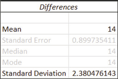Excel descriptive statistics.
The Excel descriptive statistics show the mean and standard deviation of the differences, giving us

578

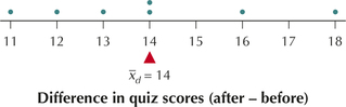Figure 10.1: FIGURE 1 Taking the differences reduces a two-sample problem to a single sample of differences.

The mean of the differences is shown as the balance point in Figure 1.

NOW YOU CAN DO

Exercises 9–14.

YOUR TURN #1

Table 2 shows the change in English quiz scores for six students before and after getting help at the English Center. Calculate the mean and the standard deviation of the differences.

Table 10.3: Table 2 English quiz scores

Student	Henrik	Ivana	Jen	Kayla	Luisa	Manuel
After	90	70	76	61	60	90
Before	92	70	75	60	58	86

(The solutions are shown in Appendix A.)

The sample of differences can be considered representative of the population of these differences, where the population represents all students who took statistics quizzes before and after visiting the Math Center. The sample mean difference is a point estimate of the population mean difference , which is the unknown mean difference in the (after – before) quiz scores for all students who visited the Math Center. Because is unknown, we need to perform hypothesis tests and construct confidence intervals to learn about its value.

Note that, in this book, always refers to sample 1 – sample 2—never sample 2 – sample 1. For example, represents the mean difference between the students' “after” scores and the “before” scores on the statistics quizzes in Table 1.

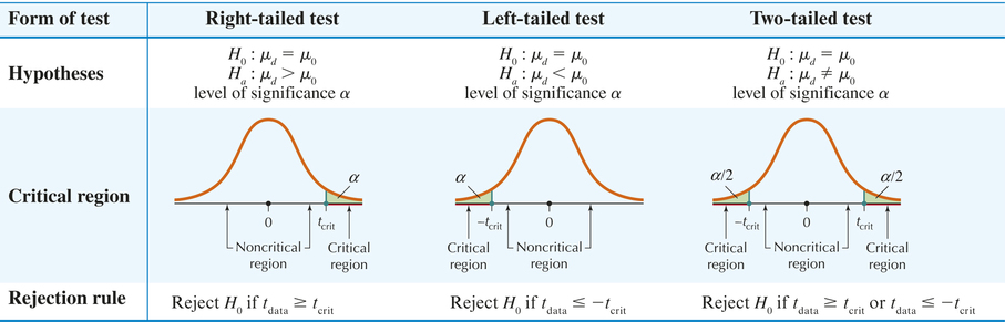
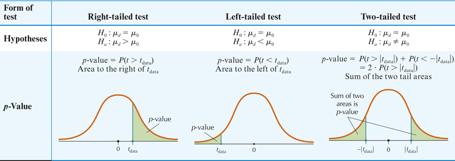
Paired Sample test for the Population Mean of the Differences : critical-value Method

For matched-pair data taken from dependent samples of two populations, find the differences to produce a random sample of the differences between the populations. You can use the test whenever either of the following conditions is met:

The population of differences is normal, or
The sample size of differences is large ().

Step 1 State the hypotheses. Use one of the hypothesis test forms in Table 3. State the meaning of .
Step 2 Find , and state the rejection rule. To find , use the table and degrees of freedom . To find the rejection rule, use Table 3.
Step 3 calculate .

which follows an approximate distribution with degrees of freedom .
Step 4 State the conclusion and the interpretation. Compare with .

Notice that we have only one sample of differences, so this procedure is very similar to the one-sample test from Section 9.4.

579

Table 10.4: Table 3 Critical regions and rejection rules for dependent sample test

EXAMPLE 3 Paired test using the critical-value method

For the Math Center data in Example 2, test, at level of significance , whether the population mean of the differences in quiz scores (after – before) is greater than zero. Or, more informally, test whether the quiz scores after visiting the Math Center are larger on average than the quiz scores before visiting the Math Center.

Solution

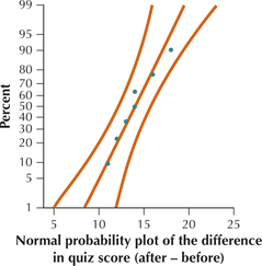
The normal probability plot of the differences shown here shows acceptable normality, allowing us to proceed with the hypothesis test.

Step 1 State the hypotheses. “Greater than” implies that , leading to the hypotheses

where represents the population mean difference in quiz scores after visiting the Math Center and before visiting the Math Center.
Step 2 Find the critical value and state the rejection rule. Use degrees of freedom. Here , so . We have a right-tailed test with , so we find our critical value by choosing the column in the table (Table D in the Appendix) with area 0.05 in one tail: . The right-tailed test tells us that our rejection rule is to reject when is greater than 1.943.
Step 3 Find . We need to calculate and .

From Example 2, we have

This gives
Step 4 State the conclusion and the interpretation. Because is greater than , we reject . There is evidence that the population mean of the differences in quiz score (after – before) is greater than zero. That is, the quiz scores after visiting the Math Center are larger on average than the quiz scores before visiting the Math Center.

NOW YOU CAN DO

Exercises 15–17.

580

YOUR TURN #2

For the set of (after – before) English quiz score differences in Table 2 (page 578), test, at level of significance , whether the population mean of the differences in quiz score (after – before) is greater than zero. (The normality of the data is fine, although you may check it with technology if you wish.)

(The solution is shown in Appendix A.)

The paired sample test may also be performed using the -value method.

Paired Sample test for the Population Mean of the Differences : -value Method

The population of differences is normal, or
The sample size of differences is large ().

Step 1 State the hypotheses and the rejection rule. Use one of the hypothesis test forms from Table 4 for a test at level of significance . State the meaning of . The rejection rule is: Reject if the -value is less than .
Step 2 calculate .

which follows an approximate distribution with degrees of freedom .
Step 3 Find the -value. If you have access to technology, use it to find the -value. Otherwise, calculate the -value using one of the test forms in Table 4.
Step 4 State the conclusion and the interpretation. Compare the - value with .

Table 10.5: Table 4 -Values for dependent sample tests

EXAMPLE 4 Paired sample test for : the -value method

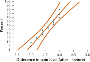
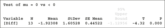
A study was performed to determine whether Reiki touch therapy was useful in the reduction of mean pain level in chronic pain sufferers, including cancer patients.³ The pain level reported by a random sample of 13 patients before and after Reiki touch therapy is shown in Table 5. Test whether a mean reduction in pain level has occurred after the Reiki therapy, using level of significance . In other words, test whether the population mean difference is less than zero, where is defined as the (after – before) difference in pain level.

reiki

581

Table 10.6: Table 5 Pain level reported by 13 patients before and after Reiki touch therapy

Patient	1	2	3	4	5	6	7	8	9	10	11	12	13
Alter	3	1	0	0	2	1	2	1	0	4	1	4	8
Before	6	2	2	3	3	4	2	5	1	6	6	4	8
Difference	-3	-1	-2	-3	-1	-3	0	-4	-1	-2	-5	0	0

Solution

For each patient, we subtract the “before” pain level from the “after” pain level to arrive at a set of differences, highlighted in Table 5. The normal probability plot of the differences indicates acceptable normality, given the small sample size. The Minitab results from the test are provided here.

Step 1 State the hypotheses and the rejection rule. We are interested in testing whether a mean reduction in pain level occurred, which would mean that the mean pain level would be lower after the Reiki therapy than before the therapy. This implies that the population mean difference in pain level, , is less than 0. Thus, from Table 4, the hypotheses are

where represents the population mean difference in pain level. We will reject if the -value < 0.05.
Step 2 Find . As provided in the Minitab results,

which follows an approximate distribution with degrees of freedom .
Step 3 Find the -value. For a left-tailed test, the -value is the area to the left of . This area is essentially 0, as shown in Figure 2 and provided by Minitab,

582

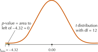Figure 10.2: FIGURE 2 The
.
Step 4 State the conclusion and the interpretation. Because , we reject . There is evidence that , thus the population mean difference in pain level (after – before) is negative. That is, there is evidence, at level of significance , that the Reiki touch therapy has worked to reduce the mean pain level for chronic pain sufferers.

NOW YOU CAN DO

Exercises 18–20.

3 Confidence Intervals for the Population Mean Difference for Dependent Samples

Recall that in Section 8.2, we used the formula to calculate the interval for the population mean . Here, to estimate the population mean of the differences , we use essentially the same formula, substituting for and for .

Confidence Interval for Population Mean Difference (Dependent Samples)

For matched-pair data taken from dependent samples of two populations, find the differences to produce a random sample of the differences between the populations. A confidence interval for , the population mean of the differences, is given by

where and represent the sample mean and sample standard deviation of the differences, respectively, of the set of paired differences, , , , …, , and where is based on degrees of freedom. This interval applies whenever either of the following conditions is met:

The population of differences is normal, or
The sample size of differences is large ().

The confidence interval for may also be expressed in the form

To construct this confidence interval, we need

583

EXAMPLE 5 Confidence interval for

Use the “before” and “after” quiz scores from Table 1 to construct a 95% confidence interval for the population mean of the differences in the statistics quiz scores.

Solution

The normality of the quiz scores was checked in Example 2. We ignore the original raw data (see Table 1) and concentrate only on the set of sample differences: {16, 13, 14, 18, 14, 11, 12}. From Example 2, we have

For 95% confidence with degrees of freedom, equals 2.447 (see the table in Appendix Table D). Using these values,

We are 95% confident that the population mean of the differences between quiz scores before and after visiting the Math Center lies between 11.7983 points and 16.2017 points. If no mean change in the quiz scores occurred, the difference would be 0, which is not in this confidence interval. Thus, we have evidence that the Math Center tutoring leads to a significant change in the mean quiz scores, with 95% confidence.

NOW YOU CAN DO

Exercises 21–26.

YOUR TURN #3

For the set of (after – before) English quiz score differences in Table 2 (page 578), construct a 90% confidence interval for the population mean of the differences in the English quiz scores.

(The solution is shown in Appendix A.)

4 Use a Interval for to Perform Tests About

Given a confidence interval for , we may perform two-tailed tests for various values of , just as we did for the single sample case in Section 9.4. The methodology is the same: if a certain value for lies outside the confidence interval for , then the null hypothesis specifying this value for would be rejected. Otherwise it would not be rejected.

EXAMPLE 6 Using a interval for to perform tests about

Example 5 provided a 95% confidence interval for the population mean of the differences between quiz scores before and after visiting the Math Center as (11.7983, 16.2017). Test, using level of significance , whether the population mean of the differences between quiz scores before and after visiting the Math Center differs from these values: (a) 15 points, (b) 16 points, (c) 17 points.

584

Solution

We state the hypotheses and determine if each proposed value lies inside or outside of the confidence interval (11.7983, 16.2017).

lies inside the interval (11.7983, 16.2017), so we do not reject (Figure 3).
lies inside the interval, so we do not reject .
lies outside the interval, so we reject .

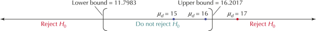Figure 10.3: FIGURE 3 Reject for values of that lie outside the confidence interval.

NOW YOU CAN DO

Exercises 27–30.

YOUR TURN #4

Use the 90% confidence interval you made for the population mean of the differences in the English quiz scores in the Your Turn #3 to test, using level of significance , whether the population differs from these values: (a) 2 points, (b) 5.6 points, (c) 5.7 points.

(The solutions are shown in Appendix A.)

Ashley:	Emily:
Brittany:	Fran:
Chris:	Greg:
Dave: