1. Find the multiple regression equation, interpret the multiple regression coefficients, and use the multiple regression equation to make predictions.
2. Calculate and interpret the adjusted coefficient of determination.
3. Perform the test for the overall significance of the multiple regression.
4. Conduct tests for the significance of individual predictor variables.
5. Explain the use and effect of dummy variables in multiple regression.
6. Apply the strategy for building a multiple regression model.

Regression analysis using a single variable and a single variable is called simple linear regression.

1. Use technology to find the multiple regression equation for predicting , using and . State the equation with a sentence.
2. State the values of the multiple regression coefficients.
3. Interpret the multiple regression coefficients for using and .
4. Use the multiple regression equation to predict the rating of a breakfast cereal with 5 mg of fiber and 10 mg of sugar.

1. A partial Minitab printout is shown in Figure 20. A partial SPSS printout is in Figure 21. The multiple regression equation is

   The estimated nutritional rating equals 52.22 points plus 2.869 times the number of grams of fiber minus 2.246 times the number of grams of sugar.

   

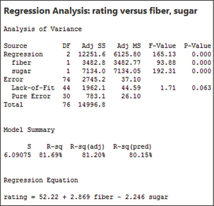   Figure 13.21: FIGURE 20 Multiple regression equation in Minitab.
   

   Figure 13.22: FIGURE 21 Multiple regression equation in SPSS.
2. The values of the multiple regression coefficients are , , and .
3. The multiple regression coefficients are interpreted as follows:
   • (y intercept). The estimated nutritional rating when there are zero grams of fiber and zero grams of sugar is 52.22.
   • . For every increase of one gram of fiber, the estimated increase in nutritional rating is 2.869 points, when the amount of sugar is held constant.
   • . For every increase of one gram of sugar, the estimated decrease in nutritional rating is 2.246 points, when the amount of fiber is held constant.

   When making predictions in multiple regression, beware of the pitfalls of extrapolation, just like those for simple linear regression. Further, in multiple regression, the values for all predictor variables must lie within their respective ranges. Otherwise, the prediction represents extrapolation, and it may be misleading.

   745

4. To find the predicted rating for a breakfast cereal with and , we plug these values into the multiple regression equation from part (a):

1. Calculate the multiple coefficient of determination for .
2. There are observations. Compute and interpret the adjusted coefficient of determination .

states that at least one of the , not that all of the .

1. Determine whether the regression assumptions have been violated.
2. Perform the test for the overall significance of the multiple regression of rating on vitamins and sodium, using level of significance .

1. Figure 22, a scatterplot of the residuals versus fitted values, contains no strong evidence of unhealthy patterns. Although the two cereals, All-Bran with Extra Fiber and Product 19, are unusual, the vast majority of the data suggest that the independence, constant variance, and zero-mean assumptions are satisfied. Figure 23 indicates that the normality assumption is satisfied.
2. The Minitab multiple regression results are provided in Figure 24.

   747

   

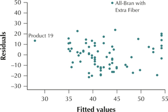   Figure 13.23: FIGURE 22 Scatterplots of residuals versus fitted values.
   

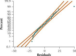   Figure 13.24: FIGURE 23 Normal probability plot of the residuals.
   

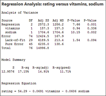   Figure 13.25: FIGURE 24 Minitab results for regression of rating on vitamins and sodium.

• Step 1 State the hypotheses and the rejection rule. We have variables, so the hypotheses are

  • . No linear relationship exists between rating and either vitamins and sodium. The overall multiple regression is not significant.
  • and . A linear relationship exists between rating and at least one of vitamins and sodium. The overall multiple regression is significant.

  Reject if the .

• Step 2 Find the statistic and the -value. These are located in the ANOVA table portion of the printout, denoted Analysis of Variance. From Figure 24, we have and . The -value represents .
• Step 3 Conclusion and interpretation. The , so we reject . There is evidence, at level of significance , for a linear relationship between rating and at least one of vitamins and sodium. The overall multiple regression is significant.

• Test 1: Test whether a significant linear relationship exists between rating and vitamins.
• Test 2: Test whether a significant linear relationship exists between rating and sodium.

• Step 1 For each hypothesis test, state the hypotheses and the rejection rule. Vitamins is , and sodium is , so the hypotheses are

  • Test 1:
    • . No linear relationship exists between rating and vitamins.
    • . A linear relationship exists between rating and vitamins.
    • Reject if the .
  • Test 2:
    • . No linear relationship exists between rating and sodium.
    • . A linear relationship exists between rating and sodium.
    • Reject if the .
• Step 2 For each hypothesis test, find the statistic and the -value. Figure 25 is an excerpt of the Minitab results from Figure 24, with the relevant statistics and -values highlighted. For Test 1, the -value represents , because it is a two-tailed test. For Test 2, the -value represents .
  • Test 1: , with -value 0.336.
  • Test 2: , with -value 0.002.
  

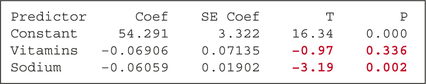  Figure 13.26: FIGURE 25 statistics and -values for the test for the significance of the variables vitamins and sodium.
• Step 3 For each hypothesis test, state the conclusion and interpretation.
  • Test 1: The , which is not . Therefore, we do not reject . There is insufficient evidence of a linear relationship between rating and vitamins when sodium is held constant. Perhaps surprisingly, the variable vitamins is not significant, meaning that the amount of vitamins in the breakfast cereal is not helpful in predicting nutritional rating.
  • Test 2: The , which is . Therefore, we reject . There is evidence of a linear relationship between rating and sodium when vitamins is held constant. The variable sodium is significant, meaning that the amount of sodium in the breakfast cereal is helpful in predicting nutritional rating.

1. Verify that the regression assumptions are met.
2. Perform a multiple regression of on and , using level of significance . Find the two regression equations, one for females and the other for males.
3. Construct a scatterplot of versus , using different-shaped points to show the different sexes. Place the two regression equations on the scatterplot.
4. Interpret the coefficient of the dummy variable .

1. Figures 26 and 27 contain no evidence of unhealthy patterns. We therefore conclude that the regression assumptions are verified.

   

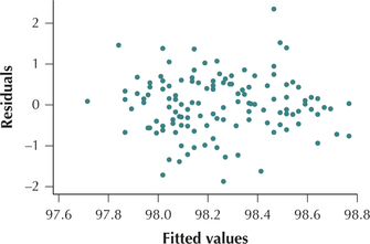   Figure 13.27: FIGURE 26 Scatterplot of residuals versus fitted values.
   

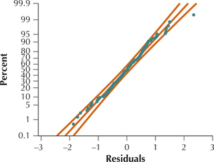   Figure 13.28: FIGURE 27 Normal probability plot of the residuals.

   750

2. Figure 28 contains the multiple regression results. The -value for the test is 0.001, which is , so we conclude that the overall regression is significant. The regression results tell us that , , and . Thus, our two regression equations are:
   • Females:
   • Males:
   

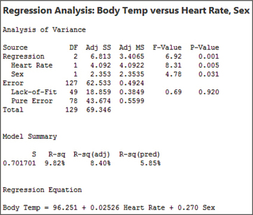   Figure 13.29: FIGURE 28 Results for multiple regression of on and .
   

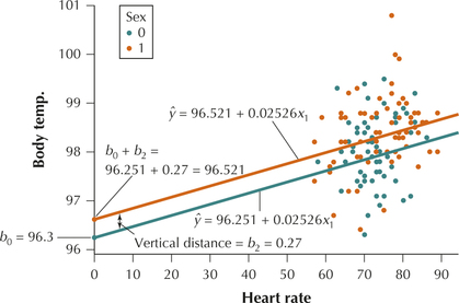   Figure 13.30: FIGURE 29 Scatterplot showing parallel regression lines when using dummy variables.
3. Figure 29 contains the scatterplot of versus , with the orange dots representing females and the blue dots representing males. The regression lines are shown, orange for females, blue for males. Note that the regression lines are parallel, because they each have the same slope . So the only difference in the lines is the intercepts.
   • For females, the intercept is .
   • For males, the intercept is simply .
4. The vertical distance between the parallel regression lines equals , as shown in Figure 29. Thus, we interpret the coefficient of the dummy variable as the estimated increase in for those observations with (females), as compared to those with (males), when heart rate is held constant. That is, for the same heart rate, females have a body temperature that is higher than that of males, by an estimated 0.27 degrees.

• Step 1 The Test.

  Construct the multiple regression equation using all relevant predictor variables. Apply the test for the significance of the overall regression, in order to make sure that a linear relationship exists between the response and at least one of the predictor variables.

  751

• Step 2 The Tests.

  Perform the tests for the individual predictors. If at least one of the predictors is not significant (that is, its -value is greater than level of significance ), then eliminate the variable with the largest -value from the model. Ignore the -value of . Repeat Step 2 until all remaining predictors are significant.

  We eliminate only one variable at a time. It may happen that eliminating one nonsignificant variable will nudge a second, formerly nonsignificant, variable into significance.

• Step 3 Verify the Assumptions.

  For your final model, verify the regression assumptions.

• Step 4 Report and Interpret Your Final Model.

  1. Provide the multiple regression equation for your final model.
  2. Interpret the multiple regression coefficients so that a nonstatistician could understand.
  3. Report and interpret the standard error of the estimate s and the adjusted coefficient of determination .

• Step 1 The Test. Figure 30 shows the Minitab results of a regression of on the set of predictor variables . The -value for the test is significant, so we know that a linear relationship exists between and at least one of the variables.

• Step 2 The test (the first time). In Figure 30, the -value for Batting Average is greater than level of significance . We therefore eliminate the Batting Average from the model. Perhaps surprisingly, a player's batting average is evidently not helpful in predicting the number of runs that player will score when all other predictors are held constant.

  752

  

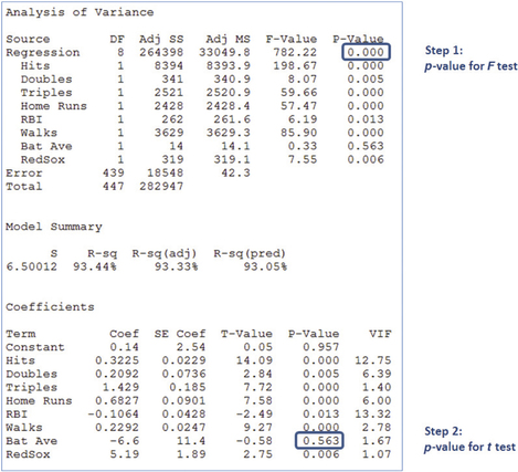  Figure 13.31: FIGURE 30 Step 1: test is significant.
  

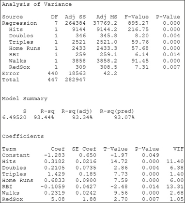  Figure 13.32: FIGURE 31 All variables are significant; we have our final model.
• Step 2 The test (the second time). We repeat Step 2 as long as there are variables with -values greater than level of significance . Figure 31 shows the results of performing the multiple regression of on all the variables except Batting Average. No further variables have -values below 0.05; therefore, no further variables are excluded from the model. In other words, we have our final model.
• Step 3 Verify the assumptions. For our final model, we now verify the regression assumptions. Figures 32 and 33 show no patterns for the bulk of the data that would indicate a violation of the regression assumptions. We therefore conclude that the regression assumptions are verified.
  

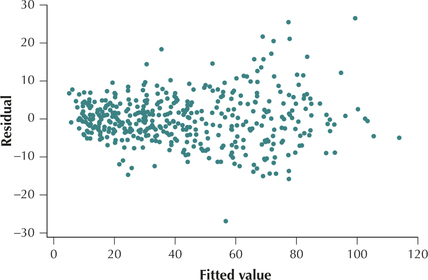  Figure 13.33: FIGURE 32 Scatterplot of residuals versus fitted values.
  

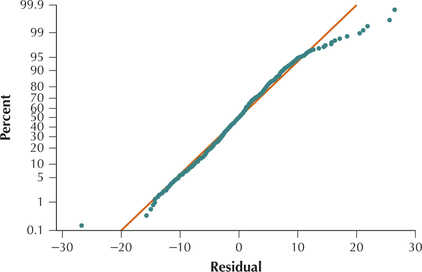  Figure 13.34: FIGURE 33 Normal probability plots of the residuals.
• Step 4 Report and interpret your final model.

  1. The multiple regression equation for the final model is shown here.

     753

  2. We interpret the coefficient for Hits, and leave to the exercises the interpretation of the other multiple regression coefficients. “For each additional hit that a player makes, the estimated increase in the number of runs that player will score is 0.3182, when all the other variables are held constant.”
  3. The standard error of the estimate for the final model is . That is, using the multiple regression equation in (a), the size of the typical prediction error will be about 6.5 runs. The value of the adjusted coefficient of determination is . In other words, 93.07% of the variability in the number of runs scored is accounted for by this multiple regression equation.