14.2 Sign Test
OBJECTIVES By the end of this section, I will be able to …
- Perform the sign test for a single population median.
- Perform the sign test for matched-pair data from two dependent samples.
- Perform the sign test for binomial data.
1 Sign Test for a Single Population Median
In Section 9.4, we learned how to perform the one-sample test for the population mean , which is a parametric test requiring either a normal population or a large sample . However, what do we do when we have neither a normal population nor a large sample? We could use either the sign test for the population median, which we learn in this section, or the signed rank test, which we learn in Section 14.3.
The sign test is a nonparametric hypothesis test in which the original data are transformed into plus or minus signs. The sign test may be conducted for (a) a single population median, (b) matched-pair data from two dependent samples, or (c) binomial data.
The following example illustrates a situation where we want to perform a hypothesis test, but the conditions are not met for performing the usual parametric hypothesis test.
14-6
EXAMPLE 1 Conditions for parametric test are not met

Since 1940, the National Weather Service has reported the annual number of hurricane-related deaths in the United States. Here is a random sample size from the population of yearly hurricane deaths:
| Year | 1959 | 1963 | 1974 | 1988 | 1999 | 2001 | 2005 | 2010 |
| Deaths | 24 | 11 | 1 | 9 | 19 | 24 | 1016 | 13 |
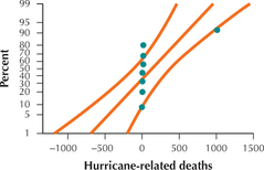
We are interested in testing whether the population mean number of hurricane-related deaths is less than 25. Figure 1 is the normal probability plot for the data. Determine whether the conditions required for the one-sample test are met.
Solution
The test may be used if the population is normal or if the sample size is at least 30. The normal probability plot shows two data values outside the bounds, indicating that the data are not normally distributed. Also, the sample of size is not at least 30. Therefore, the conditions for performing the test for the population mean are not met. (The unusual data value of 1016 hurricane-related deaths for 2005 is the result of Hurricanes Katrina and Rita.)
Fortunately, however, the required conditions for performing the sign test for the population median are less stringent than those for the test for the population mean. The sign test requires only that the sample data have been randomly selected. It is not required that the population be normally distributed. It should be noted, however, that the sign test is a hypothesis test for the population median, not the population mean.
The key concept for performing the sign test for the median is the following: each of the data values is converted to either a plus sign (+) or a minus sign (–). If there is a preponderance of plus signs to minus signs, or vice versa (depending on the form of the hypothesis test), then this is evidence against the null hypothesis.
EXAMPLE 2 Changing the data values to plus or minus signs
Suppose that we are interested in testing whether the population median number of hurricane-related deaths per year is less than 50.
- Write the null and alternative hypotheses for this test.
- Change each data value that is less than 50 to a minus sign (–), and change each data value that is greater than 50 to a plus sign (+). Ignore any data values that are equal to 50. The sample size is the total number of plus signs and minus signs.
Solution
We may write the hypotheses as
where represents the population median number of hurricane-related deaths per year.
14-7
- As shown here, we have 7 minus signs and 1 plus sign, so that our sample size is .
| Year | 1959 | 1963 | 1974 | 1988 | 1999 | 2001 | 2005 | 2010 |
| Deaths | 24 | 11 | 1 | 9 | 19 | 24 | 1016 | 13 |
| Sign | – | – | – | – | – | – | + | – |
Recall that the median of a data set is the 50th percentile and splits the data set into equal halves. Thus, if the null hypothesis were true, we would expect about half of the sample data values to lie above the median and half below, so that about half of the signs would be plus signs and about half would be minus signs. Now, only 1 of the 8 signs in this data set is a plus sign, which may indicate evidence against the null hypothesis. However, to make sure, we need to perform the sign test for the population median. The procedure for the sign test for the population median is summarized as follows.
Sign Test for the Population Median
The only requirement for performing the sign test for the population median is for the sample data to have been randomly selected. It is not necessary to have a population that is normally distributed.
- Step 1 State the hypotheses. Choose one of the forms in Table 2.Table 14.4: Table 2 Hypotheses for the sign test for the population median
Null hypothesis Alternative hypothesis Type of test Right-tailed test Left-tailed test Two-tailed test Table 14.4: Note: is the value of the population median for which a claim is being made. - Step 2 Find the critical value and state the rejection rule.
- Small-Sample Case (sample size ): Use Appendix Table I. Choose the column with the appropriate level of significance and the applicable one-tailed or two-tailed test. Then select the row with the appropriate sample size . The number in that row and column is your critical value . The rejection rule is to reject if .
- Large-Sample Case (sample size ): Use Appendix Table C, the standard normal table. The critical value for this sign test is always found in the left tail of the standard normal distribution, so that is always less than 0. For a left-tailed test or a right-tailed test, the critical value is the value of with area to the left of it. For a two-tailed test, the critical value is the value of with area to the left of it. Table 4 in Chapter 9 on page 500 contains values of for some common values of . The rejection rule is to reject if .
- Step 3 Find the value of the test statistic.
Small-Sample Case : Use Table 3 to find the test statistic .
Table 14.5: Table 3 FindingType of test Test statistic Right-tailed test Left-tailed test Two-tailed test 14-8
- Large-Sample Case : First use Table 3 to find , and then calculate the test statistic :
- Step 4 State the conclusion and the interpretation.
Compare the test statistic with the critical value, using the rejection rule. A generic interpretation is as follows. If is rejected, then state, “Evidence exists that [whatever says].” If is not rejected, then state, “There is insufficient evidence that [whatever says].”
EXAMPLE 3 Small-sample sign test for the population median
For the data from Example 2, use the sign test to determine whether the population median number of hurricane-related deaths per year is less than 50, using level of significance .
Solution
From Example 1, we know that the data come from a random sample, which is the only condition for conducting the sign test. Thus, we may proceed.
Step 1 State the hypotheses. the hypotheses are
where represents the population median number of hurricane-related deaths per year.
Step 2 Find the critical value and state the rejection rule. The total number of plus signs and minus signs is , which is not greater than 25, so we use the small-sample case. We have a one-tailed test, with and , which gives us (Figure 2). The rejection rule is to reject if .
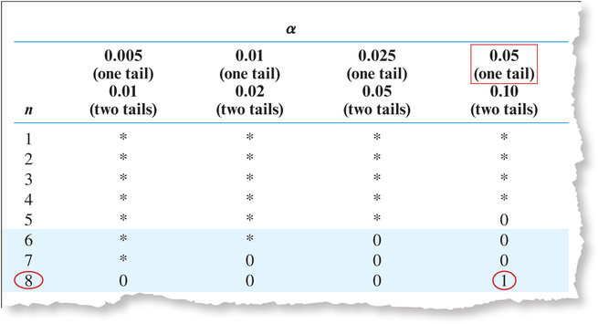 Figure 14.2: FIGURE 2 Using Appendix Table I to find the critical value .
Step 3 Find the value of the test statistic. We have a left-tailed test, and so, from Table 3, our test statistic is
14-9
Step 4 State the conclusion and the interpretation. The value of our test statistic is , which is ≤1, so we reject . Evidence exists that the population median number of hurricane-related deaths is less than 50 per year.
NOW YOU CAN DO
Exercises 9–16.
EXAMPLE 4 Large-sample sign test for the population median using technology
nutrition
The data set Nutrition (on the text website) contains information about 961 food items. The variable calories states the number of calories per serving for each food item. Consider these 961 food items to be a random sample of the population of all food items. Test whether the population median number of calories differs from 120, using level of significance .
Solution
The 961 food items are a random sample from the population of all food items, so the conditions for performing the sign test for the population median are met.
Step 1 State the hypotheses. The key words “differs from” indicate that we have a two-tailed test. The answer to the question “Differs from what?” gives us the value of .
where represents the population median calories per food item.
- Step 2 Find the critical value and state the rejection rule. We have a large sample here. Among the 961 values, there are 18 that are equal to the proposed population median . We ignore values that do not have a sign associated with them, so . We are given the level of significance , so our . We will reject if .
Step 3 Find the value of the test statistic. We use the instructions provided in the Step-by-Step Technology Guide at the end of this section. Figure 3 shows the Minitab results from the sign test for the population median. The value for “Below” is the number of minus signs, and the value for “Above” is the number of plus signs. So, we have 448 minus signs and 495 plus signs. Thus, the sample size is . From Table 3, , whichever is smaller. Thus, . We then calculate the test statistic :
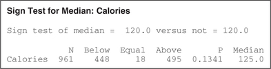 Figure 14.3: FIGURE 3 Minitab output for the sign test for the population median.
 The value of reported by Minitab does not equal the actual sample size used for the sign test. To find , we need to subtract the number of data values equal to .
14-10
- Step 4 State the conclusion and the interpretation. Because is not , we do not reject . The evidence is insufficient that the population median number of calories differs from 120 calories per serving. The Minitab output shows that the sample median equals 125 calories, which is a little bit different from , but the difference is not statistically significant.
NOW YOU CAN DO
Exercises 17–20.
2 Sign Test for Matched-Pair Data from Two Dependent Samples
In Section 10.1, we performed a hypothesis test for the population mean of the difference between two dependent samples. Recall that two samples are dependent when the subjects in the first sample determine the subjects in the second sample. For example, suppose we are interested in comparing the heights of girl-boy fraternal twins. Selecting a girl twin for the first sample automatically results in the selection of her twin brother for the second sample. The boy-girl pairs are called matched-pair samples, or paired samples.
The paired-sample test we learned in Section 10.1 required either that the population of differences be normal or that the sample size of the differences be at least 30. Here, we learn the sign test for the population median of the differences, , which requires only that the sample data be randomly selected.
The hypotheses for the population median of the differences are given in Table 4.
| Null hypothesis | Alternative hypothesis |
Type of test | Test statistic |
|---|---|---|---|
| Right-tailed test | |||
| Left-tailed test | |||
| Two-tailed test |
We may use the same methods for the matched-pair sign test that we used for the sign test for a single population median, with the following modifications:
- For each matched pair, subtract the value of the second variable from the value of the first variable.
- We are interested only in the sign of the difference found in Step 1, not the difference itself.
- Exclude ties. That is, omit any matched pairs in which the values for both variables are equal.
We illustrate the sign test for the population median of the differences using the following example.
EXAMPLE 5 Sign test for matched-pair data from two dependent samples
The National Center for Educational Statistics publishes the results from the Trends in International Math and Science Study (TIMSS). The following table contains the 2007 and 2011 average eighth-grade mathematics scores for a random sample of 12 countries. Test whether the population median math score has decreased from 2007 to 2011, using .
14-11
| Country | 2007 | 2011 | Difference (2011 – 2007) |
Sign |
|---|---|---|---|---|
| Korea | 597 | 613 | +16 | + |
| Singapore | 593 | 611 | +18 | + |
| United States | 508 | 509 | +1 | + |
| Lithuania | 506 | 502 | −4 | − |
| Hungary | 517 | 505 | −12 | − |
| Romania | 461 | 458 | −3 | − |
| Russia | 512 | 539 | +27 | + |
| Australia | 496 | 505 | +9 | + |
| Indonesia | 397 | 386 | −11 | − |
| Norway | 469 | 475 | +6 | + |
| Sweden | 491 | 484 | −7 | − |
| Malaysia | 474 | 440 | −34 | − |
Solution
The countries represent a random sample of matched-pair data, so the condition for performing the sign test for the population median of the differences is met.
Step 1 State the hypotheses. We have a left-tailed test:
where represents the population median of the differences in eighth-grade math scores from 2007 to 2011.
- Step 2 Find the critical value and state the rejection rule. The sample size is the sum of the number of plus signs and minus signs: . Because , we use the small-sample case. To find the critical value, we use Appendix Table I. We have a one-tailed test, with and , which gives us . The rejection rule is to reject if .
- Step 3 Find the value of the test statistic. From Table 3, we have .
- Step 4 State the conclusion and the interpretation. Because is not ≤2, we do not reject . There is insufficient evidence that the population median eighth-grade math score has decreased from 2007 to 2011.
NOW YOU CAN DO
Exercises 21–24.
The sign test may also be applied using the -value method and technology.
-Value Method for Conducting the Sign Test
- Step 1 State the hypotheses.
- Step 2 Find the -value using technology.
- Step 3 State the conclusion and the interpretation.
If the -value is ≤ the level of significance , reject ; otherwise, do not reject .
EXAMPLE 6 The sign test using the -value method
education
The following data set represents the education receipts (such as taxes) and the education expenditures for a random sample of 10 states. Test, using level of significance , whether the population median of the differences (receipts − expenditures) per state differs from zero.
14-12
| State | Receipts ($ millions) |
Expenditures ($ millions) |
Difference |
|---|---|---|---|
| Florida | 28,208 | 26,832 | 1,376 |
| California | 73,272 | 68,045 | 5,227 |
| New Jersey | 20,032 | 19,938 | 94 |
| Alabama | 7,000 | 6,540 | 460 |
| Minnesota | 10,280 | 10,191 | 89 |
| Indiana | 11, 9 9 6 | 11, 315 | 681 |
| Maine | 2,458 | 2,458 | 0 |
| New York | 41,800 | 42,895 | −1,095 |
| Mississippi | 4,3 41 | 3,945 | 396 |
| Ohio | 24,259 | 21,237 | 3,022 |
Solution
The states represent a random sample of matched-pair data. We may thus proceed with the sign test for the population median of the differences.
Step 1 State the hypotheses.
where represents the population median of the differences in education receipts minus expenditures per state.
- Step 2 Find the -value using technology. We use the instructions provided in the Step-by-Step Technology Guide at the end of this section. The Minitab output shown in Figure 4 and the JMP output shown in Figure 5 provide the -value for this hypothesis test: . Note that one state (Maine) has education receipts equal to expenditures, so that the difference for Maine equals zero. Maine is thus omitted, and the -value is based on the other nine states left in the sample.
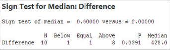 Figure 14.4: FIGURE 4 Minitab output for the sign test for the population median.
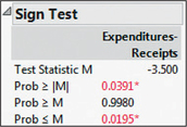 Figure 14.5: FIGURE 5 JMP output for the sign test for the population median.
 - Step 3 State the conclusion and the interpretation. The -value 0.0391 is less than the level of significance , so we reject . Evidence exists that the population median difference between education receipts and expenditures differs from zero.
3 Sign Test for Binomial Data
In Section 9.5, we performed the test for the population proportion of successes . Here, we learn about the sign test for binomial data, which is a special case of the test for the population proportion for . Recall that a variable is binomial if it takes only two possible values, such as on/off, up/down, in/out. For example, the following example looks at the numbers of spam emails and nonspam emails processed by a university spam filter. When using the sign test, spam emails are represented by plus (+) signs, and nonspam emails are represented by minus (−) signs. Table 5 contains the hypotheses for the sign test for binomial data. Note that the hypothesized population proportion is always .
14-13
| Null hypothesis | Alternative hypothesis |
Type of test | Test statistic |
|---|---|---|---|
| Right-tailed test | |||
| Left-tailed test | |||
| Two-tailed test |
We use the same methods for the sign test for binomial data that we used for the sign test for a single population median. However, only the large-sample case is used , because only when the sample size is large does the Central Limit Theorem apply.
EXAMPLE 7 Sign test for binomial data
The National Center for Health Statistics reports that 50% of Americans take at least one prescription drug per month. Suppose that a random sample of 100 Americans shows 67 who took at least one prescription drug per month. Test whether the proportion of Americans who take at least one prescription drug per month has increased, using .
Solution
Because the sample of Americans has been selected randomly and , we may proceed. We represent people taking at least one prescription drug per month by plus (+) signs and people taking no prescription drugs by minus (–) signs.
Step 1 State the hypotheses.
where represents the population proportion of Americans taking at least one prescription drug per month.
- Step 2 Find the critical value and state the rejection rule. The sample size is greater than 25, so we may use the large-sample case. Using Table 4 in Chapter 9 (page 500) for level of significance , we have . We will reject if .
- Step 3 Find the value of the test statistic. From Table 5, . Thus, . We then calculate the test statistic :
- Step 4 State the conclusion and the interpretation. Because is , we reject . Evidence exists that the population proportion of Americans taking at least one prescription drug per month has increased.
NOW YOU CAN DO
Exercises 25–26.
14-14
vehicles

 Has Median Gas Mileage increased?
The data set in Table 6 represents a random sample of vehicles that were manufactured in model years 2007 and 2014 and matched so that the various engine characteristics (displacement, number of cylinders, and so on) are the same for each model in the two years.1 Thus, we are dealing with matched-pair data, comparing the combined miles per gallon (that is, city and highway mpg) for the same vehicles from two different years. Use the sign test to test whether the population median of the difference in gas mileage (2014 – 2007) is greater than zero, using level of significance .
| Make | Model | Combined mpg for 2007 |
Combined mpg for 2014 |
Difference (2014 – 2007) |
Sign |
|---|---|---|---|---|---|
| Chevrolet | Tahoe | 17 | 17 | 0 | None |
| Chevrolet | Suburban | 17 | 17 | 0 | None |
| Dodge | Caravan | 21 | 20 | −1 | − |
| Ford | Explorer | 17 | 19 | 2 | + |
| Ford | F150 Pickup | 16 | 18 | 2 | + |
| Ford | Mustang | 17 | 19 | 2 | + |
| Ford | Taurus | 23 | 21 | −2 | − |
| GMC | Savana Cargo | 17 | 16 | −1 | − |
| GMC | Yukon XL | 17 | 17 | 0 | None |
| Subaru | Forester | 25 | 27 | 2 | + |
| Subaru | Impreza | 25 | 27 | 2 | + |
| Subaru | Legacy | 25 | 27 | 2 | + |
| Toyota | Corolla | 36 | 35 | −1 | − |
| Toyota | Tacoma | 21 | 23 | 2 | + |
Solution
The vehicles represent a random sample, so the condition for performing the sign test for the population median of the differences is met.
Step 1 State the hypotheses. Here, we have a right-tailed test:
where represents the population median of the differences in miles per gallon (2014 – 2007).
- Step 2 Find the critical value and state the rejection rule. The sample size is the sum of the number of plus signs and minus signs. There are 7 plus signs and 4 minus signs, so that . Because , we use the small-sample case. To find the critical value, we use Appendix Table I. We have a one-tailed test, with and , which gives us . The rejection rule is to reject if .
- Step 3 Find the value of the test statistic. From Table 5, we have .
- Step 4 State the conclusion and the interpretation. Because , we do not reject . The evidence is insufficient to conclude that the population median of the differences (2014 – 2007) is greater than zero. In other words, the evidence is insufficient to conclude that the population median vehicle gas mileage has increased from 2007 to 2014.
We return to this Case Study in Section 14.3, when we apply the Wilcoxon signed rank test to the same question.