3.4 Measures of Relative Position and Outliers
155
OBJECTIVES By the end of this section, I will be able to …
- Calculate -scores, and explain why we use them.
- Detect outliers using the -score method.
- Find percentiles and percentile ranks for both small and large data sets.
- Compute quartiles and the interquartile range.
In this section, we learn about measures of relative position, which tell us the position that a particular data value has relative to the rest of the data set. For example, a prestigious nursing school may grant admission to only the top 10% of applicants. How high a score would you need to enter? This is one type of question we will answer in this section.
1 -scores
Recall that the standard deviation is a common measure of the variability, or spread, of a data set, and its value is interpreted as a typical deviation from the mean.
Our first measure of relative position is the -score. Recall that the standard deviation is a common measure of the variability, or spread, of a data set. The -score indicates how many standard deviations a particular data value is from the mean. If the -score is positive, then the data value is above the mean. If the -score is negative, then the data value is below the mean.
-score
The -score for a particular data value from a sample is
where is the sample mean, and is the sample standard deviation.
The -score for a particular data value from a population is
where is the population mean, and is the population standard deviation. -scores can be positive or negative.
- A positive -score indicates that the data value, , lies above the mean.
- A negative -score implies that lies below the mean.
- A -score equal to zero indicates that equals the mean.
In this section, we will use the sample -score unless otherwise indicated.
EXAMPLE 21 Calculating -scores, given data values
People thinking about applying for a loan should take care that they maintain a healthy credit score, which comes from paying monthly bills on time and paying off previous loans without any problems. Figure 22 shows a histogram of the credit scores of over 150,000 loan applicants (Source: Data Mining and Predictive Analytics, by Daniel Larose and Chantal Larose, Wiley, 2015). The mean of this population of credit scores is , with a standard deviation of . Calculate and interpret the -scores for the following loan applicants:
156
- Jasmine has been taking care to pay all her bills on time, so she has a healthy credit score of 740.
- Jeremy was laid off, defaulted on a previous loan, and so has a credit rating of 439.
- May-Chang always pays her bills on time and has already paid off several loans. Her credit score is 817.
Solution
Note that here we have population values, with and .
- Jasmine's credit score is . Her -score is
We interpret Jasmine's -score of 1 to mean that her credit score of 740 lies 1 standard deviation above the mean . See Figure 22.
- The -score for Jeremy's credit score of 439 is
Jeremy's credit score lies 3.3 standard deviations below the mean.
- The -score for May-Chang's credit score of 817 is
May-Chang's credit score lies 2.1 standard deviations above the mean.
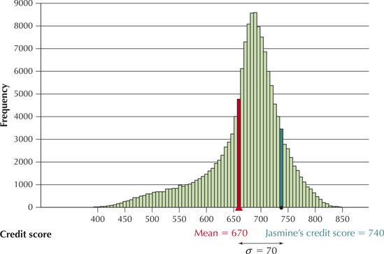 Figure 3.22: FIGURE 22 Jasmine's -score of 1 places her 1 standard deviation above the mean.
NOW YOU CAN DO
Exercises 7–18.
YOUR TURN #11
The IBM Digital Analytics Benchmark reports that tablet users (for tablets such as the iPad) spent a mean of $96 per order for their 2013 online holiday shopping. Assume that the standard deviation is $40. Find the -scores for the following tablet-using holiday shoppers:
- Austin spent $136 on video games.
- Brian spent $16 on music downloads.
- Courtney spent $256 on gifts for her friends.
(The solutions are shown in Appendix A.)
157
Alternatively, we may be given a -score and asked to find its associated data value, . To do so, use the following formulas.
Note: We arrive at these formulas simply by taking the -score formula and using algebra to solve for .
Given a -score, to find its associated data value :
where is the population mean, is the sample mean, is the population standard deviation, and is the sample standard deviation.
EXAMPLE 22 Finding data values given -scores
Continuing with the credit score data from Example 21, find the credit scores (the x-values) associated with the following -scores:
- −1
- 0
- 0.5
Solution
We have population data, with , .
- For a -score of −1, we have
A credit score of 600 is associated with a -score of −1, and therefore lies 1 standard deviation below the mean.
- For a -score of 0, we have
As noted earlier, a -score of zero exactly equals the mean .
- For a -score of 0.5, we have
A -score of 0.5 is associated with a credit score of 705.
NOW YOU CAN DO
Exercises 19–30.
YOUR TURN #12
Continuing the online holiday shopping example from Your Turn #11 on page 156, find the spending amounts associated with the following -scores.
- David's -score was 21.5. How much did he spend?
- Emily had a -score of 2.5. What was her spending amount?
- Frances had a -score of zero. What did she spend?
(The solutions are shown in Appendix A.)
EXAMPLE 23 Using the -score to compare data from different data sets
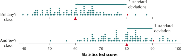
Andrew is bragging to his friend Brittany that he did better than she did on the last statistics test. Andrew got a 90, while Brittany got an 80. Andrew's class mean was 80, with a standard deviation of 10. Brittany's class mean was 60, with a standard deviation of 10. The professors in both classes grade “on a curve” using -scores. Who did better relative to his or her class?
158
Solution
Brittany can use -scores to show that she did better relative to her class. Figure 23 shows comparative dotplots of the scores in the two classes. The red dots represent Brittany's and Andrew's scores. Brittany found her -score by subtracting her class mean from her score of 80 and then dividing by the standard deviation :
z-Scores enable the data analyst to compare data values from two different distributions.
Brittany's -score is 2. What does that mean? It means that Brittany scored 2 standard deviations above the mean of 60. Brittany then found the -score for Andrew:
Andrew's -score was 1, which means that Andrew scored 1 standard deviation above the mean. From Figure 23, we can observe that Andrew's exam score of 90 lies closer to the mean exam score of 80 for his class. That is, the arrow is shorter for Andrew than for Brittany. Finally, note that 10 of the 100 students who took the exam in his class did better than he did, whereas only two did better than Brittany in her class. So, relative to her class, Brittany did better than Andrew, even though Andrew got a higher score. The -scores allowed her to compare their grades, even though they were in different classes.
NOW YOU CAN DO
Exercises 31 and 32.
YOUR TURN #13
Continuing the online holiday shopping example from Your Turn #11, the IBM Digital Analytics Benchmark also reported that cell phone users spent a mean of an average of $85 per order for their 2013 online holiday shopping. Assume the standard deviation is $40. Gisele is a tablet user, whereas Hong is a cell phone user. They both spent the same amount for an online holiday shopping order: $120. Who spent more, relative to his or her group?
(The solution is shown in Appendix A.)
2 Detecting Outliers using the -score Method
Note: If an outlier is detected, it does not automatically follow that it should be discarded. Outliers often indicate the presence of something interesting going on in the data that would call for further investigation. On the other hand, it could simply be a typo. The analyst should check with the data source.
An outlier is a data value that is very much greater than or less than the mean. It may represent a data entry error, or it may be genuine data. One way of identifying an outlier is to determine whether it is farther than 3 standard deviations from the mean, that is, its -score is less than −3 or greater than 3.
Guidelines for Identifying Outliers
- A data value whose -score lies in the following range is considered not unusual:
159
- A data value whose -score lies in either of the following ranges may be considered moderately unusual:
- A data value whose -score lies in either of the following ranges may be considered an outlier:
EXAMPLE 24 Detecting outliers using the -score method
For the three loan applicants in Example 21 on page 155, determine whether each of their credit scores represents an outlier.
Solution
- Jasmine's -score is 1, which lies in the range, . Therefore, Jasmine's credit rating is not considered unusual.
- Jeremy's -score is −3.3, which is . Thus, Jeremy's credit score may be considered an outlier.
- May-Chang's -score is 2.1, which lies in the range, . Thus, May-Chang's credit score may be considered moderately unusual.
NOW YOU CAN DO
Exercises 33–44.
YOUR TURN #14
Refer to the -scores you calculated for Austin, Brian, and Courtney in Your Turn #11 on page 156. Determine whether each of their spending amounts represents an outlier.
(The solutions are shown in Appendix A.)
In Section 3.5, we will learn about the IQR method of detecting outliers.
3 Percentiles and Percentile Ranks
The next measure of relative position we consider is the percentile, which shows the location of a data value relative to the other values in the data set.
percentile
Let be any integer between 0 and 100. The th percentile of a data set is the data value at which percent of the values in the data set are less than or equal to this value.
Some analysts prefer to define the pth percentile to be a data value at which at least percent of the values in the data set are less than or equal to this value, and at least percent of the values are greater than or equal to this value.
EXAMPLE 25 Meaning of a percentile
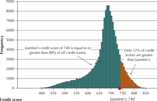
Jasmine's credit score of 740 represents the 88th percentile of the 150,000 credit scores. What does “88th percentile” mean?
Solution
To say that 740 is the 88th percentile means that 88% of all credit scores fell at or below Jasmine's credit score of 740. We call the percentile a measure of relative position because it indicates the position of Jasmine's credit score relative to all other credit scores. Figure 24 indicates the position of Jasmine's credit score relative to the rest of the loan applicants.
160
For large data sets, calculation of the percentiles is best left to computers. However, for small data sets, we can use the following step-by-step method to calculate the related position of any percentile.
- Step 1 Sort the data into ascending order (from smallest to largest).
- Step 2 Calculate
where is the particular percentile you wish to calculate, and is the sample size.
- Step 3
- If is an integer (a whole number with no decimal part), the th percentile is the mean of the data values in positions .
- If is not an integer, round up to the next integer and use the value in this position.
 These steps do not give the value of the th percentile itself, but rather the position of the th percentile in the data set when the data set is in ascending order.
EXAMPLE 26 Finding percentiles
Table 22 contains the value of international exports for a sample of 12 states for the month of June 2014, expressed in millions of dollars. Find the 75th percentile of the exports.
| State | VA | NC | NJ | GA | PA | OH | MI | FL | LA | IL | WA | NY |
|---|---|---|---|---|---|---|---|---|---|---|---|---|
| Exports ($ millions) |
1.6 | 2.7 | 3.3 | 3.5 | 3.5 | 4.6 | 4.7 | 4.8 | 5.0 | 5.8 | 7.5 | 7.7 |
161
stateexports
Solution
- Step 1 Sort the data into ascending order. Fortunately, Table 22 is already presented in ascending order of exports.
- Step 2 The particular percentile we wish to calculate is the 75th percentile, so . Our data set includes 12 values, so . Calculate
So,
- Step 3 Here, is an integer, so the 75th percentile is the mean of the data values in positions 9 and 10.
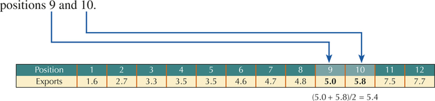
Counting from left to right, the data value in the 9th position is Louisiana's 5.0, and the data value in the 10th position is Illinois' 5.8. The mean of these two values is 5.4. Thus, the 75th percentile is 5.4, representing $5.4 million in exports.
NOW YOU CAN DO
Exercises 45–56.
YOUR TURN #15
Jason is doing a class project on some of the lowest-rated movies on the movie database IMDB. He will use movies whose ratings are in the 20th percentile or lower. A sample of movie ratings follows. Calculate the 20th percentile rating.
| 8.7 | 5.4 | 7.1 | 3.6 | 1.9 | 5.7 | 4.2 | 9.3 | 2.5 |
(The solution is shown in Appendix A.)
Remember: A percentile is a data value, whereas a percentile rank is a percentage.
The percentile rank of a data value, , equals the percentage of values in the data set that are less than or equal to . In other words:
EXAMPLE 27 Finding percentile ranks
For the state export data in the previous example, calculate the percentile ranks for the following export values:
- $5.4 million
- $3.4 million
Solution
- Here, . Nine states have -values at or below 5.4, so the percentile rank of a state with $5.4 million in exports is
Note that, therefore, $5.4 million represents the 75th percentile of state exports.
162
- Here . Three states have -values at or below 3.4, so the percentile rank of a state with $3.4 million in exports is
Thus, $3.4 million represents the 25th percentile of state exports.
NOW YOU CAN DO
Exercises 57–68.
YOUR TURN #16
For the movie rating data from Your Turn #15 on page 161, calculate the percentile rank for a movie with a rating of 9.0.
(The solution is shown in Appendix A.)
4 Quartiles and the interquartile range
Just as the median divides the data set into halves, the quartiles are the percentiles that divide the data set into quarters (Figure 25).
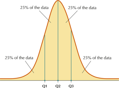
The Quartiles
The quartiles of a data set divide the data set into four parts, each containing 25% of the data.
- The first quartile (Q1) is the 25th percentile.
- The second quartile (Q2) is the 50th percentile, that is, the median.
- The third quartile (Q3) is the 75th percentile.
For small data sets, the division may be into four parts of only approximately equal size.
163
EXAMPLE 28 Finding the quartiles for a small data set
Note: It may be helpful to note that the phrase third quartile is akin to the phrase three quarters, which is 75%, representing the 75th percentile. Also, the phrase first quartile is akin to the phrase one quarter, which is 25%, representing the 25th percentile.
In Example 26 (page 160), we found the 75th percentile of the export data to be $5.4 million. By definition, the 75th percentile is the third quartile Q3. Therefore, this export value of $5.4 million is also the third quartile (Q3) of the export values. Now calculate the first quartile and the median (second quartile) of export values.
Solution
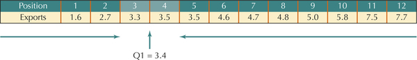
To find the quartiles, we use the steps for finding percentiles (page 160). First, arrange the data set in ascending order, which they already are in Table 22.
Here, . To find Q1, plug into the equation , where . We get . Since 3 is an integer, we know that the 25th percentile is the mean of the export values in the 3rd and 4th positions. New Jersey's export value of 3.3 is in the 3rd position, while Georgia's export value of 3.5 is in the 4th position. Since , we get the 25th percentile of the export data to be 3.4, representing $3.4 million in exports (Figure 26).
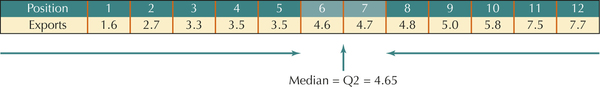
To find the median (the second quartile, Q2), plug into your steps for finding the percentiles: . Since 6 is an integer, we know that the 50th percentile is the mean of the export data in the 6th and 7th positions, that is, 4.6 and 4.7. Since , the 50th percentile of the export data is 4.65, representing $4.65 million in exports (Figure 27). This agrees with the method we learned for finding the median, on page 112.
The quartiles may be found on the TI-83/84 by using the instructions for descriptive statistics shown on page 117.
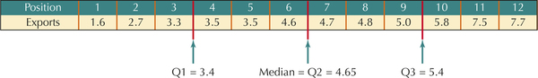
In Example 26, we determined that the 75th percentile was 5.4. Therefore, the quartiles for the export data are , , and . Note that these quartiles divide the data set into four equal sections, with three observations each (Figure 28).
NOW YOU CAN DO
Exercises 69–76.
164
YOUR TURN #17
As a follow-up to his project, Jason is dividing movie ratings into Great (at or above Q3), Good (from Q2 to Q3), Mediocre (from Q1 to Q2), and Awful (lower than Q1). Find Q1, Q2, and Q3 from the following sample of movie ratings.
| 8.7 | 5.4 | 7.1 | 3.6 | 1.9 | 5.7 | 4.2 | 9.3 | 2.5 |
(The solution is shown in Appendix A.)
Of course, for small data sets, the division into quarters is not always exact. For example, what if our data set consisted of 11 states instead of 12? Eleven data values cannot be divided equally into four quarters. In this case, therefore, the quartiles would divide the data set into four sections of approximately equal size. However, for large data sets, which the data analyst most often encounters, this becomes less of an issue.
EXAMPLE 29 Finding quartiles of a large data set: Cholesterol levels in food
nutrition
Note: Minitab uses a different way to calculate the quartiles than the way we have learned, which results in different values than our hand-calculation methods. However, for large data sets, the difference is minimal.
The U.S. Department of Agriculture recommends a diet low in cholesterol to reduce the risk of heart disease. The data set Nutrition contains information on the cholesterol content (in milligrams) of 961 different foods. Find the mean, standard deviation, and quartiles.
Solution
The Minitab descriptive statistics for the cholesterol data are shown in Figure 29. Note that the mean cholesterol content is 32.55 mg and the standard deviation is about 120 mg. A standard deviation that is much larger than the mean may be associated with strongly skewed distributions. Compare the value for the mean with the values for the quartiles as follows:
- Q1, the first quartile, or 25th percentile, is 0 mg of cholesterol.
- The median, or Q2, the second quartile (50th percentile), is also 0 mg of cholesterol.
- Q3, the third quartile, or 75th percentile, is 20 mg of cholesterol.
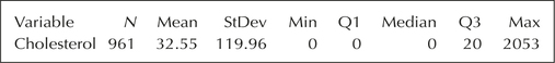 Figure 3.29: FIGURE 29 Descriptive statistics for the cholesterol data.
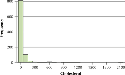
Figure 30 shows that the data distribution is extremely right-skewed. Only a few foods have over 1000 mg cholesterol, and another handful have over 500 (see data on disk). Therefore, it appears that we have outliers in this data set. What is the effect of these outliers on the mean and standard deviation? Does the mean represent a truly typical cholesterol content level for the data set, or is its value unduly increased by the outliers? Let's find out.
165
Developing Your Statistical Sense
The Mean Is Not Always Representative
Note that the median is 0 mg of cholesterol, meaning that at least half of the food items tested by the U.S. Department of Agriculture in this data set had no cholesterol at all. We are intrigued by this result and ask Minitab to provide us with a frequency distribution for the cholesterol content, along with the cumulative percentages (“CumPct”). Figure 31 provides a portion of this frequency distribution, with the following results:
- 61.91% of the food items have no cholesterol at all, which explains why Q1 and the median are both zero.
- The 75th percentile, Q3, is verified as 20 mg cholesterol.
- The 81st percentile of the data set is 32 mg cholesterol.
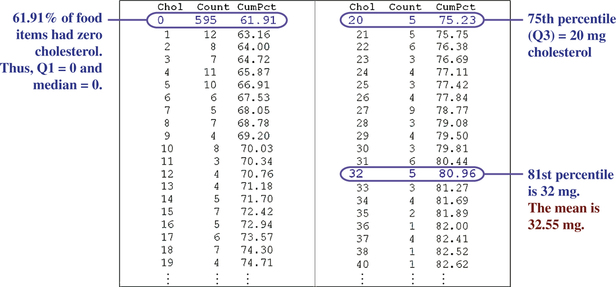 Figure 3.31: FIGURE 31 Partial frequency distribution of cholesterol content.
Think about these results for a moment. We found that the 81st percentile is 32 mg cholesterol. In other words, 81% of the food items have a cholesterol content of 32 mg or less. And yet, this 32 mg is still less than the mean cholesterol content, reported by Minitab to be 32.55 mg. In other words, the mean of this data set is larger than 81% of the data values in the data set.
It seems clear, therefore, that the mean 32.55 mg cannot be considered as typical or representative of the data set. Its value has been exaggerated by the presence of the outliers, to such an extent that it is now larger than 81% of the data. We need another, more robust measure of center—one that is resistant to the undue influence of outliers, such as the median. Here, the value of the median is 0 mg cholesterol. An argument may certainly be made that this is indeed typical and representative of the data set, because 61.91% of the food items have no cholesterol content at all.
Recall from Section 3.2 that the variance and standard deviation are measures of spread that are sensitive to the presence of extreme values. A more robust (less sensitive) measure of variability is the interquartile range, or IQR.
166
interquartile range
The interquartile range (IQR) is a robust measure of variability. It is calculated as
The interquartile range is interpreted to be the spread of the middle 50% of the data.
The Latin word inter means “between,” so the interquartile range is the difference between the quartiles Q3 and Q1. The IQR represents how spread out the “middle half ” of the data set is. A larger IQR implies a greater degree of variability, or spread, in the data set. The IQR ignores both the highest 25% and the lowest 25% of the data set, so it is completely unaffected by outliers and is thus quite robust.
EXAMPLE 30 Finding the interquartile range
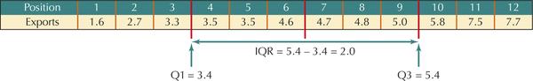
In Example 28, we found that, for the export data, and . Find the IQR for the export data, and explain what it means.
Solution
Because and , the , which represents $2 million. We would say that the middle 50%, or middle half, of the export data ranged over $2 million (Figure 32).
NOW YOU CAN DO
Exercises 77 and 78.
YOUR TURN #18
Find the interquartile range for Jason's follow-up movie ratings project.
| 8.7 | 5.4 | 7.1 | 3.6 | 1.9 | 5.7 | 4.2 | 9.3 | 2.5 |
(The solution is shown in Appendix A.)
 What If Scenario
For the state export data, consider the following two scenarios, and explain how the change would affect the quartiles and the IQR.
- New York's imports are increased by an unknown amount.
- Illinois' imports are increased by an unknown amount.
Solution
The IQR pays attention only to the middle half of the data, and it ignores what goes on in the upper 25% and the lower 25%.
- New York is the maximum value for the data set, so any change in New York's exports would leave the quartiles unaffected; therefore, the IQR would also be unaffected.
- Recall that Illinois' $5.8 million was used in the calculation of Q3, which is . Increasing Illinois' exports would therefore increase the value of Q3; therefore, the IQR would also increase. However, Q1 and the median would remain unaffected.
167