Section 3.2 Exercises
Unless a data set is identified as a population, you can assume that it is a sample.
CLARIFYING THE CONCEPTS
Question 3.114
1. Explain what a deviation is. (p. 128)
3.2.1
Deviation for a data value gives the distance the value is from the mean.
Question 3.115
2. What is the interpretation of the value of the standard deviation? (p. 132)
Question 3.116
3. State one benefit and one drawback of using the range as a measure of spread. (p. 128)
3.2.3
Benefit—simple to calculate, Drawbacks—quite sensitive to extreme values, does not use all of the data values.
Question 3.117
4. True or false: If two data sets have the same mean, median, and mode, then they are identical. (p. 127)
Question 3.118
5. What is one benefit of using the standard deviation instead of the range as a measure of spread? What is one drawback? (p. 128)
3.2.5
Benefit—uses all of the numbers in a data set. Drawback—can be time-consuming to calculate.
Question 3.119
6. Which measure of spread represents the mean squared deviation for the population? (p. 130)
Question 3.120
7. True or false: Chebyshev's Rule provides exact percentages. (p. 138)
3.2.7
False
141
Question 3.121
8. When can the sample standard deviation, , be negative? (p. 133)
Question 3.122
9. When does the sample standard deviation, , equal zero? (p. 133)
3.2.9
When all of the data values are the same
Question 3.123
10. When may the Empirical Rule be used? (p. 135)
PRACTICING THE TECHNIQUES
 CHECK IT OUT!
| To do | Check out | Topic |
|---|---|---|
| Exercises 11a–16a | Example 9 | Range |
| Exercises 11c–16c | Example 10 | Calculating deviations |
| Exercises 11d–16d | Example 11 | Population variance |
| Exercises 11e–16e | Example 12 | Population standard deviation |
| Exercises 17–22 | Example 13 | Sample variance and sample standard deviation |
| Exercises 23–30 | Example 15 | Empirical Rule |
| Exercises 31–38 | Example 16 | Chebyshev's Rule |
For the population data in Exercises 11–16, do the following:
- Compute the range.
- Find the population mean, .
- Calculate the deviations, .
- Compute the population variance, .
- Find the population standard deviation, .
Question 3.124
11. State exports to other countries are shown in the table for the population of all New England states, for the month of June 2014, expressed in billions of dollars.
| State | Exports | State | Exports |
|---|---|---|---|
| Connecticut | 1.4 | New Hampshire | 0.4 |
| Maine | 0.3 | Rhode Island | 0.2 |
| Massachusetts | 2.4 | Vermont | 0.3 |
3.2.11
(a) 2.2 (b) $0.83 billion (c) –$0.63 billion, –$0.53 billion, –$0.53 billion, –$0.43 billion, $0.57 billion, $1.57 billion (d) 0.6556 billions of dollars squared (e) $0.8097 billion dollars
Question 3.125
12. The number of wins for each baseball team in the population of the American League West division for 2013 is shown in the table.
| Team | Wins | Team | Wins |
|---|---|---|---|
| Oakland Athletics | 96 | Seattle Mariners | 71 |
| Texas Rangers | 91 | Houston Astros | 51 |
| Los Angeles Angels | 78 |
Question 3.126
13. The table provides the motor vehicle theft rate for the population of the top 10 countries in the world for motor vehicle theft, for 2012. The theft rate equals the number of motor vehicles stolen in 2012 per 100,000 residents.
| Country | Theft rate | Country | Theft rate |
|---|---|---|---|
| Italy | 208.0 | Greece | 100.2 |
| France | 174.1 | Norway | 94.1 |
| USA | 167.8 | Netherlands | 75.2 |
| Sweden | 117.2 | Spain | 75.1 |
| Belgium | 106.0 | Cyprus | 66.0 |
3.2.13
(a) 142 motor vehicles stolen per 100,000 people (b) 118.37 motor vehicles stolen per 100,000 people (c) 89.63, 55.73 49.43, –1.17. –12.37, –18.17, –24.27, –43.17, –43.27, –52.37 motor vehicles stolen per 100,000 people (d) 2113.4821 motor vehicles stolen per 100,000 people squared (e) 45.97 motor vehicles stolen per 100,000 people
Question 3.127
14. The National Center for Education Statistics sponsors the Trends in International Mathematics and Science Study (TIMSS). The table contains the mean science scores for the eighth-grade science test for the population of all Asian-Pacific countries that took the exam.
| Country | Science Score |
Country | Science Score |
|---|---|---|---|
| Singapore | 578 | Australia | 527 |
| Taiwan | 571 | New Zealand | 520 |
| South Korea | 558 | Malaysia | 510 |
| Hong Kong | 556 | Indonesia | 420 |
| Japan | 552 | Philippines | 377 |
Question 3.128
15. The table contains the number of petit larceny cases for the population of all police precincts in South Manhattan in 2013.
| Precinct | Petit larcenies | Precinct | Petit larcenies |
|---|---|---|---|
| 1 | 2014 | 10 | 995 |
| 5 | 1288 | 13 | 2094 |
| 6 | 1555 | 14 | 4551 |
| 7 | 584 | 17 | 823 |
| 9 | 1607 | 18 | 2071 |
3.2.15
(a) 3967 petit larceny cases (b) 1758.2 petit larceny cases (c) 255.8, –470.2, –203.2, –1174.2, –151.2, –763.2, 335.8, 2792.8, –935.2, 312.8 petit larceny cases (d) 1,119,682.96 petit larceny cases squared (e) 1058.15 petit larceny cases
Question 3.129
16. The table contains the number of criminal trespass cases for the population of all police precincts in South Manhattan in 2013.
| Precinct | Criminal trespass |
Precinct | Criminal trespass |
|---|---|---|---|
| 1 | 108 | 10 | 207 |
| 5 | 105 | 13 | 135 |
| 6 | 113 | 14 | 340 |
| 7 | 233 | 17 | 74 |
| 9 | 219 | 18 | 120 |
For the sample data in Exercises 17–22, do the following:
- Calculate the sample variance.
- Compute the sample standard deviation.
- Interpret the sample standard deviation.
142
Question 3.130
17. A sample of the state export data from Exercise 11 is provided in the table.
| State | Exports |
|---|---|
| Connecticut | 1.4 |
| Massachusetts | 2.4 |
| Rhode Island | 0.2 |
3.2.17
(a) 1.2133 billion dollars squared (b) $1.10 billion (c) For this sample of state export data, the typical difference between a state's export amount and the mean export amount is $1.10 billion.
Question 3.131
18. A sample from the baseball data in Exercise 12 is shown here.
| Team | Wins |
|---|---|
| Texas Rangers | 91 |
| Los Angeles Angels | 78 |
| Seattle Mariners | 71 |
Question 3.132
19. A sample from the motor vehicle theft data in Exercise 13 is as follows.
| Country | Theft rate |
|---|---|
| Italy | 208.0 |
| USA | 167.8 |
| Greece | 100.2 |
3.2.19
(a) 2967.7733 motor vehicles stolen per 100,000 people squared (b) 54.48 motor vehicles stolen per 100,000 people (c) For this sample of motor vehicle theft data, the typical difference between a country's motor vehicle theft rate and the mean motor vehicle theft rate is 54.48 motor vehicles stolen per 100,000 people.
Question 3.133
20. A sample from the science score data in Exercise 14 is given here.
| Country | Science score |
|---|---|
| South Korea | 558 |
| Hong Kong | 556 |
| Japan | 552 |
| Australia | 527 |
Question 3.134
21. The following sample is taken from the petit larceny data in Exercise 15.
| Precinct | Petit larcenies |
|---|---|
| 1 | 2014 |
| 6 | 1555 |
| 9 | 1607 |
| 14 | 4551 |
| 17 | 823 |
3.2.21
(a) 2,046,275 petit larceny cases squared (b) 1430.48 petit larceny cases (c) For this sample of New York precincts, the typical difference between a precinct's number of petit larceny cases and the mean number of petit larceny cases is 1430.48 petit larceny cases.
Question 3.135
22. A sample taken from the criminal trespass data in Exercise 16 is as follows.
| Precinct | Criminal trespasses |
|---|---|
| 1 | 108 |
| 7 | 233 |
| 14 | 340 |
| 18 | 120 |
For Exercises 23–26, use the following information. A data distribution is bell-shaped, with a mean of 50 and a standard deviation of 5. Use the Empirical Rule to approximate the percentage of data.
Question 3.136
23. Between 45 and 55
3.2.23
About 68%
Question 3.137
24. Between 40 and 60
Question 3.138
25. Between 35 and 65
3.2.25
About 99.7%
Question 3.139
26. Less than 45
For Exercises 27–30, use the following information. A data distribution is bell-shaped, with a mean of 0 and a standard deviation of 1. Use the Empirical Rule to approximate the percentage of data.
Question 3.140
27. Between −1 and 1
3.2.27
About 68%
Question 3.141
28. Greater than 2
Question 3.142
29. Less than −2
3.2.29
About 2.5%
Question 3.143
30. Between −2 and 2
For Exercises 31–34, use the following information. A data set has an unknown distribution, with a mean of 20 and a standard deviation of 2. Use Chebyshev's Rule to estimate the minimum possible percentage of data.
Question 3.144
31. Between 16 and 24
3.2.31
At least 75%
Question 3.145
32. Between 14 and 26
Question 3.146
33. Between 12 and 28
3.2.33
At least 93.75%
Question 3.147
34. Between 13 and 27
For Exercises 35–38, use the following information. A data set has an unknown distribution, with a mean of 20 and a standard deviation of 5. If possible, use Chebyshev's Rule to estimate the minimum possible percentage of data.
Question 3.148
35. Between 0 and 40
3.2.35
At least 93.75%
Question 3.149
36. Between 5 and 35
Question 3.150
37. Between 12.5 and 27.5
3.2.37
At least 55.56%
Question 3.151
38. Between 15 and 25
APPLYING THE CONCEPTS
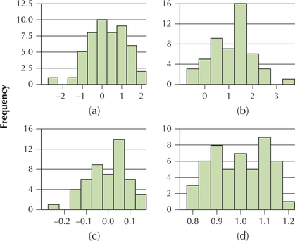
Question 3.152
39. Match the histograms in (a)–(d) to the statistics in (i)–(iv).
- ,
- ,
- ,
- ,
3.2.39
(i)—(d); (ii)—(b); (iii)—(c); (iv)—(a)
143
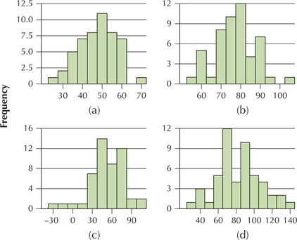
Question 3.153
40. Match the histograms in (a)–(d) to the statistics in (i)–(iv).
- ,
- ,
- ,
- ,
For the following exercises, make sure to state your answers in the proper units, such as “years” or “years squared.”
Video game Sales. The Chapter 1 Case Study looked at video game sales for the top 30 video games. The following table contains the total sales (in game units) and weeks on the top 30 list for a sample of five randomly selected video games. Use this information for Exercises 41 and 42.
Question 3.154
41. Find the following measures of spread for total sales:
- Range
- Sample variance
- Sample standard deviation
3.2.41
(a) 1.5 million game units (b) 0.327 million game units squared (c) 0.5718 million game units
Question 3.155
videogamereg
42. Calculate the following measures of spread for the number of weeks on the top 30 list:
- Range
- Sample variance
- Sample standard deviation
| Video game | Total sales in millions of units |
Weeks on list |
|---|---|---|
| Super Mario Bros. U for WiiU | 1.7 | 78 |
| NBA 2K14 for PS4 | 0.6 | 27 |
| Battlefield 4 for PS3 | 0.9 | 29 |
| Titanfall for XBoxOne | 1.2 | 10 |
| Yoshi's New Island for 3DS | 0.2 | 10 |
 Darts and the DJIA. The following table contains a random sample of eight days from the Chapter 3 Case Study data set, indicating the stock market gain or loss for the portfolio chosen by the random darts, as well as the DJIA gain or loss for that day. Use this information for Exercises 43 and 44.
Question 3.156
43. Find the following measures of spread for the darts:
- Range
- Sample variance
- Sample standard deviation
3.2.43
(a) 69.6 (b) 522.7286 (c) 22.86
Question 3.157
dartsdjia
44. Calculate the following measures of spread for the DJIA:
- Range
- Sample variance
- Sample standard deviation
| Darts | DJIA |
|---|---|
| −27.4 | −12.8 |
| 18.7 | 9.3 |
| 42.2 | 8 |
| −16.3 | −8.5 |
| 11.2 | 15.8 |
| 28.5 | 10.6 |
| 1.8 | 11.5 |
| 16.9 | −5.3 |
Age and Height. The following table provides a random sample from the Chapter 4 Case Study data set body_ females, showing the age and height of the eight women. Use this information for Exercises 45 and 46.
Question 3.158
45. Find the following measures of spread for age:
- Range
- Sample variance
- Sample standard deviation
3.2.45
(a) 21 years (b) 47.5536 years squared (c) 6.90 years
Question 3.159
ageheight
46. Calculate the following measures of spread for height:
- Range
- Sample variance
- Sample standard deviation
| Age | Height |
|---|---|
| 40 | 63.5 |
| 28 | 63.0 |
| 25 | 64.4 |
| 34 | 63.0 |
| 26 | 63.8 |
| 21 | 68.0 |
| 19 | 61.8 |
| 24 | 69.0 |
144
Saturated Fat and Calories. The table contains the calories and saturated fat in a sample of 10 food items. Use this information for Exercises 47 and 48.
Question 3.160
47. Find the following measures of spread for calories:
- Range
- Sample variance
- Sample standard deviation
3.2.47
(a) 316 calories (b) 13,520.1778 calories squared (c) 116.28 calories
Question 3.161
satfatcorr
48. Calculate the following measures of spread for saturated fat:
- Range
- Sample variance
- Sample standard deviation
| Food item | Calories | Grams of saturated fat |
|---|---|---|
| Chocolate bar (1.45 ounces) | 216 | 7.0 |
| Meat & veggie pizza (large slice) |
364 | 5.6 |
| New England clam chowder (1 cup) |
149 | 1.9 |
| Baked chicken drumstick (no skin, medium size) |
75 | 0.6 |
| Curly fries, deep-fried (4 ounces) |
276 | 3.2 |
| Wheat bagel (large) | 375 | 0.3 |
| Chicken curry (1 cup) | 146 | 1.6 |
| Cake doughnut hole(one) | 59 | 0.5 |
| Rye bread (1 slice) | 67 | 0.2 |
| Raisin bran cereal (1 cup) | 195 | 0.3 |
Video Game Sales. Refer to the video game sales data in Exercises 41 and 42 for Exercises 49–52.
Question 3.162
49. The sample variance of sales was expressed in “game units squared.” Do you find this concept easy to understand? Which measure do you find to be more easily understood and interpreted for these data, the variance or the standard deviation?
3.2.49
No, standard deviation
Question 3.163
50. Consider the histogram of total units sold for all the top 30 video games.
- Is the distribution bell-shaped?
- Can we apply the Empirical Rule?
- Can we apply Chebyshev's Rule?
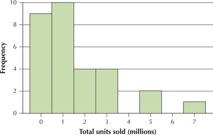
Question 3.164
51. Use the sample of size five and Chebyshev's Rule to find the minimum percentage of total sales that are between 0.0048 million and 1.8352 million.
3.2.51
At least 60.94%
Question 3.165
52. Refer to Table 3 of Chapter 1 on page 8. Calculate the actual proportion of total sales that are between 0.0048 million and 1.8352 million. Does this fit the answer you got using Chebyshev's Rule?
Darts and the DJIA. Refer to the darts and DJIA data in Exercises 43 and 44 for Exercises 53–56.
Question 3.166
53. Based on your measures of spread in Exercises 43 and 44, which stock market return reflects greater variability, the darts or the DJIA?
3.2.53
The darts
Question 3.167
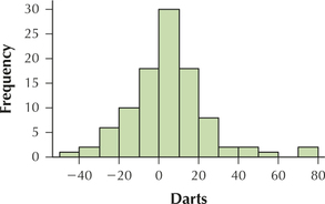
54. The histogram shows the population distribution of the stock market changes for the darts. Can we live with the assumption that the distribution is bell-shaped?
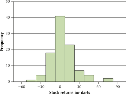
Question 3.168
55. Based on the sample of size 8, use the Empirical Rule to approximate the percentage of darts stock returns that lie between −13.41 and 32.31.
3.2.55
About 68%
Question 3.169
56. Can the Empirical Rule tell us what approximate percentage of the darts stock returns lie between −1.98 and 20.88? Explain.
Age and Height. Refer to the age and height data in Exercises 45 and 46 for Exercises 57–60.
Question 3.170
57. The histogram shows the population distribution of the women's ages.
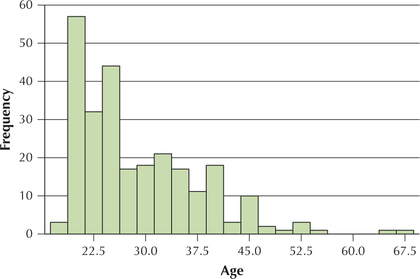
145
- Is the distribution bell-shaped?
- Can we apply the Empirical Rule?
- Can we apply Chebyshev's Rule?
3.2.57
(a) No (b) No (c) Yes
Question 3.171
58. Based on the sample of size 8, use Chebyshev's Rule to find the minimum percentage of the women's ages that lie between 16.78 and 37.48.
Question 3.172
59. The histogram shows the population distribution of the women's heights.
- Though it's not perfect, can we live with the assumption that the distribution is bell-shaped?
- Can we apply the Empirical Rule?
- Can we apply Chebyshev's Rule?
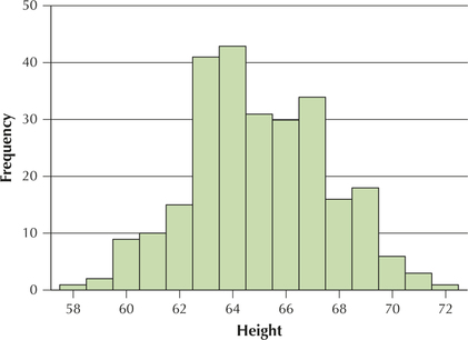
3.2.59
(a) Yes (b) Yes (c) Yes
Question 3.173
60. Based on the sample of size 8, use the Empirical Rule to approximate the percentage of the women's heights that lie between 59.449 inches and 69.677 inches.
Saturated Fat and Calories. Refer to the food data in Exercises 47 and 48 for Exercises 61 and 62.
Question 3.174
61. The histogram contains the grams of saturated fat for the 10 foods in the sample.
- Is the distribution bell-shaped?
- Can we apply the Empirical Rule?
- Can we apply Chebyshev's Rule?
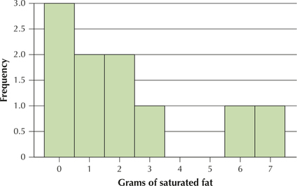
3.2.61
(a) No (b) No (c) Yes
Question 3.175
62. Use Chebyshev's Rule to find the minimum percentage of food items with saturated fat between −1.51 and 5.75.
(Note that, because grams of saturated fat cannot be negative, this is the same as between 0 and 5.75.)
Fuel Economy. Refer to Table 7 on page 123 to answer Exercises 63–65. The data represent a sample.
Question 3.176
63. Find the following measures of spread for the number of cylinders:
- Range
- Variance
- Standard deviation
3.2.63
(a) 8 cylinders (b) 9.6 cylinders2 (c) 3.098 cylinders
Question 3.177
64. Find the following measures of spread for the engine size:
- Range
- Variance
- Standard deviation
Question 3.178
65. Find the following measures of spread for the fuel economy:
- Range
- Variance
- Standard deviation
3.2.65
(a) 30 mpg (b) 116 mpg2 (c) 10.770 mpg
Ant Size. Use the following information for Exercises 66 and 67. A study compared the size of ants from different colonies. The masses (in milligrams) of samples of ants from two different colonies are shown in the accompanying table.4
| Colony A | Colony B | ||
|---|---|---|---|
| 109 | 134 | 148 | 115 |
| 120 | 94 | 110 | 101 |
| 94 | 113 | 110 | 158 |
| 61 | 111 | 97 | 67 |
| 72 | 106 | 136 | 114 |
Question 3.179
antcolony
66. Calculate the range for each ant colony.
- Which has the greater range?
- Which colony has the greater variability according to the range?
Question 3.180
antcolony
67. Calculate the standard deviation for each colony.
- Which has the greater standard deviation?
- Which colony has the greater variability according to the standard deviation? Does this concur with your answer from the previous exercise?
- Without calculating the variances, say which colony has the greater variance. How do you know this?
3.2.67
Colony A = 21.91, Colony B = 26.35 (a) Colony B (b) Colony B; yes (c) Colony B, because it has the larger standard deviation
Question 3.181
68. Computational Formula for the Population Variance and Standard Deviation: Wins in Baseball.
The following table provides the number of wins for all the teams in the American League East Division for the 2013 season, which we can consider to be a population.
146
| Team | Wins |
|---|---|
| Boston Red Sox | 97 |
| Tampa Bay Rays | 92 |
| Baltimore Orioles | 85 |
| New York Yankees | 85 |
| Toronto Blue Jays | 74 |
An alternative computational formula for the population variance is as follows:
- Use the computational formula to find the population variance for the number of wins.
- Use your result from (a) to find the population standard deviation for the number of wins.
Note: means that you square each data value and then add up the squared data values, and means that you add up all the data values and then square the sum.
Question 3.182
69. Computational Formula for the Sample Variance and Standard Deviation. Refer to the previous exercise. Suppose a random sample of size from these teams yields the New York Yankees, the Tampa Bay Rays, and the Baltimore Orioles.
An alternative computational formula for the sample variance is as follows:
- Use the computational formula to find the sample variance for the number of wins.
- Use your result from (a) to find the sample standard deviation for the number of wins.
- Interpret your result from (b).
3.2.69
(a) 16.33 wins squared (b) 4.04 wins
Question 3.183
70. Challenge Exercise. Refer to the table in Exercise 68. Suppose we are taking a sample of size .
- Which sample of two teams will yield the largest sample standard deviation? Explain your reasoning.
- Which sample of two teams will yield the smallest sample standard deviation? Explain your reasoning.
Question 3.184
71. Empirical Rule: October in Santa Monica. The National Climate Data Center reports that the mean October temperature in Santa Monica, California, is 63 degrees Fahrenheit, with a standard deviation of 3 degrees. Suppose the data distribution is bell-shaped. If possible, estimate the percentage of October days with temperatures within the following ranges. If not possible, explain why.
- Between 60 and 66 degrees
- Between 57 and 69 degrees
- Between 55 and 71 degrees
3.2.71
(a) About 68% (b) About 95% (c) Can't do, the Empirical Rule does not say what percent of the data values lie within 2.67 standard deviations of the mean.
Question 3.185
72. Empirical rule: Energy Consumption. The U.S. Department of Energy reports that the mean annual energy consumption per person in the United States is 1400 watts. Assume that the standard deviation is 200 watts and the data distribution is bell-shaped. Estimate the percentage of Americans with energy consumption within the following ranges.
- Between 1200 and 1600 watts
- Between 1000 and 1800 watts
- Above 1000 watts
Question 3.186
73. Chebyshev's Rule. Refer to Exercise 71. Suppose that we did not know that the October temperature in Santa Monica is bell-shaped. If possible, find minimums for (a)–(c) in Exercise 71.
3.2.73
(a) Can't do (b) At least 75% (c) At least 85.94%
Question 3.187
74. Chebyshev's Rule. Refer to Exercise 72. Suppose that we did not know that the annual energy consumption is bell-shaped. If possible, find minimums for (a)–(c) in Exercise 72.
Energy Consumption. Refer to Table 16, which shows the per capita energy consumption (watts per person) for samples of countries on three continents for Exercises 75–78.
| Asia | Europe | North America |
|---|---|---|
| China 447 | Germany 861 | USA 1402 |
| Japan 774 | France 804 | Canada 1871 |
| South Korea 1038 | United Kingdom 622 | Mexico 131 |
Question 3.188
energyconsumption
75. Construct dotplots of the energy consumption for each continent. Which continent would you say has the greatest spread (variability)? Why?
3.2.75
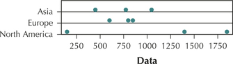
North America, because the dots for North America are more spread out than the dots for Asia and Europe.
Question 3.189
energyconsumption
76. Find the range and variance of the per capita energy consumption for each of the continents. Do your findings agree with your judgment from the previous exercise?
Question 3.190
energyconsumption
77. Without performing any calculations, use your results from the previous exercise to state which continent has (a) the largest standard deviation, and (b) the smallest standard deviation.
3.2.77
(a) North America (b) Europe
Question 3.191
energyconsumption
 78. Now suppose we omit Mexico from the data.
- Without recalculating them, describe how this would affect the values of the measures of spread you found for the North American countries.
- Now recalculate the three measures of spread for the North American countries. Was your judgment in (a) supported?
Women's Volleyball Team Heights. Refer to Table 10 on page 126 for Exercises 79–81.
Question 3.192
79. Suppose a new player joins the NCU team. She is 7 feet tall (84 inches) and replaces the 72-inch-tall player.
- Would you expect the standard deviation to go up or down, and why?
- Now find the standard deviation for the team including the new player. Was your intuition correct?
3.2.79
(a) Increase because the contribution of a value of 84 to the computation is greater than the contribution of a value of 72. (b) 7.27; yes.
147
Question 3.193
80. Linear Transformations. Add 4 inches to the height of each player on the WMU team.
- Recalculate the range and standard deviation.
- Formulate a rule for the behavior of these measures of variability when a constant (such as 4) is added to each member of the data set.
Question 3.194
81. Linear transformations. Starting with the original data, double the height of each player on the NCU team.
- Recalculate the range and standard deviation.
- Formulate a rule for the range and standard deviation when the data values are doubled.
3.2.81
(a) Range = 12; standard deviation = 4.9 (b) Multiplying each value in a data set by a constant will increase the value of the original range or standard deviation by a factor of the constant.
Coefficient of Variation. The coefficient of variation enables analysts to compare the variability of two data sets that are measured on different scales. The coefficient of variation (CV) itself does not have a unit of measure. Larger values of CV indicate greater variability or spread. The coefficient of variation is given as
Use this measure of variability for Exercises 82 and 83.
Question 3.195
82. Coefficient of Variation for Fuel Economy Data.
Refer to Table 7 on page 123.
- Calculate the coefficient of variation for the following variables: cylinders, engine size, and city mpg.
- According to the coefficient of variation, which variable has the greatest spread? The least variability?
Question 3.196
83. Coefficient of Variation for Energy Consumption.
Refer to Table 16 on page 146.
- Calculate the coefficient of variation for the per capita energy consumption for each continent.
- According to the coefficient of variation, which continent has the greatest spread? Does this agree with your measures of spread from Exercise 76?
3.2.83
Asia: 39.32%, Europe: 16.37%, North America: 79.34% Yes
Mean absolute Deviation. Recall that the variance and standard deviation use squared deviations because the mean deviation for any data set is zero. Another way to avoid negative deviations offsetting positive ones is to use the absolute value of the deviations. The mean absolute deviation (MAD) is a measure of spread that looks at the average of the absolute values of the deviations:
Use this measure of variability for Exercises 84 and 85.
Question 3.197
84. Mean absolute Deviation for the fuel economy Data. Refer to Table 7 on page 123.
- Find the mean absolute deviation for cylinders, engine size, and city mpg.
- According to the mean absolute deviation, which variable has the greatest variability? The least variability?
Question 3.198
85. Mean absolute Deviation for energy Consumption. Refer to Table 16 on page 146.
- Calculate the mean absolute deviation for each continent.
- According to the mean absolute deviation, which continent has the greatest spread? Does this agree with your measures of spread from Exercise 76?
3.2.85
(a) Asia: 204 watts per person; Europe: 93.56 watts per person; North America: 669.11 watts per person (b) North America, yes
Coefficient of Skewness. The coefficient of skewness quantifies the skewness of a distribution. It is defined as
Most skewness values lie between 23 and 3. Negative values of skewness are associated with left-skewed distributions, whereas positive values are associated with right-skewed distributions. Values close to zero indicate distributions that are nearly symmetric. Use this information for Exercises 86–88.
Question 3.199
86. Coefficient of Skewness. For the following distributions, compute the coefficient of skewness and comment on the skewness of the distribution.
- , ,
- , ,
- , ,
- , ,
- , ,
- , ,
Question 3.200
87. What is the coefficient of skewness for any distribution where the mean equals the median, regardless of the nonzero value of the standard deviation?
3.2.87
0
Question 3.201
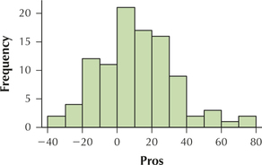
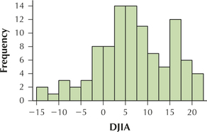
88.
Coefficient of Skewness for the Case Study Data. The median price change for the professional analysts is 9.60, the median for the dart throwers is 3.25, and the median for the DJIA is 7.00. Use this information, along with the information in Figure 21 on page 140 to answer the following.
- Calculate the coefficient of skewness for each of the Pros, the Darts, and the DJIA.
- Comment on the skewness of each distribution.
BRINGING IT ALL TOGETHER
In Exercises 89 and 90, we bring together all the measures of spread we have learned in the chapter and the new ones we learned in the exercises.
Question 3.202
89. Fuel Economy Data. You calculated the range, variance, and standard deviation for this data in Exercises 63–65. You calculated the coefficient of variation in Exercise 82 and the mean absolute deviation in Exercise 84. Use this information to do the following.
- Construct a table of the five measures of dispersion (range, sample variance, sample standard deviation, coefficient of variation, and mean absolute deviation) for the number of cylinders, the engine size, and the city mpg.
148
- Which measures of dispersion suggest that the city mpg is the most dispersed variable? Engine size? Number of cylinders?
3.2.89
(a)
| Range | Sample variance |
Sample standard deviation |
Coefficient of variation |
Mean absolute deviation |
|
|---|---|---|---|---|---|
| Cylinders | 8 | 9.6 | 3.098 | 51.64% | 2 |
| Engine size | 4.9 | 3.078 | 1.754 | 52.89% | 1.189 |
| City mpg | 30 | 116 | 10.770 | 44.88% | 8.333 |
(b) City mpg: Range, Sample variance, Sample standard deviation, Mean absolute deviation. Engine size: Coefficient of variation; Cylinders: None of them.
Question 3.203
90. Energy Consumption Data. You calculated the range and variance for this data in Exercise 76. You calculated the coefficient of variation in Exercise 83 and the mean absolute deviation in Exercise 85. Use this information to do the following:
- Using the variance, calculate the standard deviation energy consumption for each continent.
- Construct a table of the five measures of spread (range, sample variance, sample standard deviation, coefficient of variation, and mean absolute deviation) for each continent.
- Do the measures of spread agree on which distribution has the greatest variability?
- Bringing together all your statistics about measures of spread, what is your conclusion about the variability in Europe, compared with the other two continents?
CONSTRUCT YOUR OWN DATA SETS
Question 3.204
91. Construct two data sets, A and B, that you make up on your own, so that the range of A is greater than the range of B. Verify this.
3.2.91
Answers will vary.
Question 3.205
92. Construct two data sets, A and B, that you make up on your own, so that the standard deviation of A is greater than the range of B. Verify this.
Question 3.206
93. Construct two data sets, A and B, that you make up on your own, so that the mean of A is greater than the mean of B, but the standard deviation of B is greater than that of A. Verify this.
3.2.93
Answers will vary.
Question 3.207
94. Construct two data sets, A and B, that you make up on your own, so that the mean of A is greater than the mean of B, and the standard deviation of A is greater than that of B. Verify this.
Question 3.208
95. Construct two data sets, A and B, that you make up on your own, so that the range of A is greater than the range of B, but the standard deviation of B is greater than that of A. Verify this. (Hint: Remember the sensitivity of the standard deviation to extreme values.)
3.2.95
Answers will vary.
WORKING WITH LARGE DATA SETS
The Professionals versus the Darts. We will assess how well the Empirical Rule performs, using the Chapter 3 Case Study data set. Open the Darts data set. Use technology to do the following.
 darts
darts
Question 3.209
darts
96. Find the mean and standard deviation for each of the Pros, the Darts, and the DJIA.
Question 3.210
darts
97. Construct histograms of each of the Pros, the Darts, and the DJIA. Conclude that we can live with the assumption of a bell-shaped distribution for all three groups.
3.2.97
Question 3.211
darts
98. For the Pros, do the following:
- Calculate the following quantities: , , , , , and .
- State what approximate percentages lie within those intervals, according to the Empirical Rule.
- Count how many stock returns actually lie within each of those intervals. Divide these counts by the population size 100 to obtain the actual percentages.
- Compare the approximate percentages estimated by the Empirical Rule with the actual percentages from the population data.
Question 3.212
darts
99. Repeat the same comparison (a)–(d) from Exercise 98, but this time for the Darts.
3.2.99
(a)
(b) About 68% of the stock returns lie between −14.87 and 23.91. About 95% of the stock returns lie between –34.26 and 43.3. About 99.7% of the stock returns lie between –53.65 and 62.69. (c) 76% of the stock returns lie between –14.87 and 23.91. 94% of the stock returns lie between –34.26 and 43.3. 98% of the stock returns lie between –53.65 and 62.69. (d) The actual percentages that lie within each interval are close to the approximate percentages given by the Empirical Rule.
Question 3.213
darts
100. Repeat the same comparison (a)–(d) from Exercise 98, but this time for the DJIA.