Section 4.2 Exercises
CLARIFYING THE CONCEPTS
Question 4.99
1. What is the objective of regression analysis? (p. 209)
4.2.1
To approximate the relationship between two numerical variables using the regression line and the regression equation
Question 4.100
2. What is the regression equation? (p. 210)
Question 4.101
3. Describe how we use the regression equation to make predictions. (p. 213)
4.2.3
We can find the predicted value of by plugging a given value of into the regression equation and simplifying.
Question 4.102
4. Explain the difference between and . (p. 214)
Question 4.103
5. Describe what is meant by extrapolation. (p. 215)
4.2.5
Extrapolation is the process of making predictions based on -values that are beyond the range of the -values in our data set.
Question 4.104
6. What is the relationship between the slope of the regression line and the correlation coefficient? (p. 210)
218
PRACTICING THE TECHNIQUES
 CHECK IT OUT!
| To do | Check out | Topic |
|---|---|---|
| Exercises 7–12, and 13a–24a |
Example 6 | Calculating the regression coefficients. |
| Exercises 13b–24b | Example 7 | Interpreting slope and intercept |
| Exercises 25a–36a | Example 9 | Making predictions |
| Exercises 25b–36b | Example 10 | Calculating and interpreting prediction errors |
| Exercises 25c–36c | Example 11 | Extrapolation |
Exercises 7–12 refer to scatterplots in the Section 4.1 exercises. For each indicated scatterplot, state whether the slope of the regression line would be positive, negative, or near zero.
Question 4.105
7. Exercise 21
4.2.7
Negative
Question 4.106
8. Exercise 22
Question 4.107
9. Exercise 23
4.2.9
Positive
Question 4.108
10. Exercise 24
Question 4.109
11. Exercise 25
4.2.11
Negative
Question 4.110
12. Exercise 26
For Exercises 13–24, do the following:
- Calculate the slope and the intercept of the regression line. Write the regression equation.
- Interpret the values for and .
Question 4.111
13.
| 10 | 20 | 30 | 40 | |
| 2 | 5 | 9 | 12 |
4.2.13
(a) (b) For each increase of 1 unit, the estimated value of increases by 0.34 unit. When the estimated value of is −1.5.
Question 4.112
14.
| 0 | 2 | 4 | 6 | |
| 50 | 60 | 50 | 40 |
Question 4.113
15.
| −5 | −4 | −3 | −2 | −1 | |
| 10 | 18 | 18 | 26 | 26 |
4.2.15
(a) (b) For each increase of 1 unit, the estimated value of increases by 4 units. When the estimated value of is 31.6.
Question 4.114
16.
| −3 | −1 | 1 | 3 | 5 | |
| −25 | −35 | −40 | −45 | −50 |
Question 4.115
17.
| 5 | 10 | 15 | 20 | 25 | 30 | |
| 7 | 8 | 8 | 8 | 7 | 8 |
4.2.17
(a) (b) For each increase of 1 unit, the estimated value of increases by 0.0114 unit. When the estimated value of is 7.4667.
Question 4.116
18.
| 6 | 7 | 8 | 9 | 11 | 13 | |
| 9 | 9 | 9 | 9 | 9 | 9 |
Question 4.117
19.
| −70 | −60 | −50 | −40 | −30 | −20 | −10 | 0 | |
| 5 | 10 | 15 | 20 | 20 | 15 | 10 | 5 |
4.2.19
(a) (b) For each increase of 1 unit, the estimated value of remains 12.5. When the estimated value of is 12.5.
Question 4.118
20.
| −30 | −23 | −15 | −12 | −1 | 5 | 14 | 29 | |
| 103 | 88 | 76 | 62 | 54 | 47 | 30 | 20 |
Question 4.119
21. The heights (in inches) and weights (in pounds) of a sample of five women are recorded.
| 66 | 122 |
| 67 | 133 |
| 69 | 153 |
| 68 | 138 |
| 65 | 125 |
4.2.21
(a) (b) For each increase of 1 inch, the estimated weight increases by 7.2 pounds. When inches, the estimated weight is −348.2 pounds.
Question 4.120
22. The number of days absent from a class, and the course grade.
| 0 | 95 |
| 2 | 90 |
| 4 | 85 |
| 6 | 70 |
| 8 | 60 |
Question 4.121
23. The cost of a repair job and the number of hours spent on the repair.
| 2 | 120 |
| 3 | 180 |
| 5 | 230 |
| 8 | 350 |
| 10 | 380 |
4.2.23
(a) (b) For each increase of 1 hour of labor, the estimated cost of the repairs increases by $32.61. When hours of labor, the estimated cost of the repairs is $69.38.
Question 4.122
24. Attendance at a baseball game (in thousands), and the amount of rainfall at a baseball stadium that day (in inches).
| 0.0 | 40 |
| 0.0 | 42 |
| 0.1 | 38 |
| 0.5 | 30 |
| 1.0 | 20 |
For Exercises 25–36, do the following for the indicated data:
- Predict the value of for the given value of .
- Calculate and interpret the prediction error.
- State whether or not the prediction represents extrapolation.
Question 4.123
25. Data from Exercise 13;
4.2.25
(a) (b) . The data point lies above the regression line, so the actual -value of 9 is greater than the predicted -value of 8.7. (c) Does not represent extrapolation
Question 4.124
26. Data from Exercise 14;
Question 4.125
27. Data from Exercise 15;
4.2.27
(a) (b) . The data point lies below the regression line, so the actual -value of 10 is less than the predicted -value of 11.6. (c) Does not represent extrapolation
Question 4.126
28. Data from Exercise 16;
Question 4.127
29. Data from Exercise 17;
4.2.29
(a) (b) can't be found (c) Represents extrapolation
219
Question 4.128
30. Data from Exercise 18;
Question 4.129
31. Data from Exercise 19;
4.2.31
(a) (b) The data point lies below the regression line, so the actual -value of 5 is less than the predicted -value of 12.5. (c) Does not represent extrapolation
Question 4.130
32. Data from Exercise 20;
Question 4.131
33. Data from Exercise 21;
4.2.33
(a) (b) . The data point lies below the regression line, so the actual weight of 138 pounds is less than the predicted weight of 141.4 pounds. (c) Does not represent extrapolation
Question 4.132
34. Data from Exercise 22;
Question 4.133
35. Data from Exercise 23;
4.2.35
(a) (b) can't be found (c) Represents extrapolation
Question 4.134
36. Data from Exercise 24;
APPLYING THE CONCEPTS
For Exercises 37–51, do the following for the indicated data sets from the Section 4.1 exercises:
- Calculate the slope and the intercept of the regression line.
- State the regression equation in words.
- Interpret the value for the slope of the regression line, in terms of the variables from the particular exercise.
- Interpret the value for the intercept of the regression line, in terms of the variables from the particular exercise.
Question 4.135
videogamereg
37. Video Game Sales. The Chapter 1 Case Study looked at video game sales for the top 30 video games. The following table contains the total sales (, in game units) and weeks on the top 30 list of 5 randomly chosen video games.
| Video game | Total sales in millions of units |
Weeks |
|---|---|---|
| Super Mario Bros. U for WiiU | 1.7 | 78 |
| NBA 2K14 for PS4 | 0.6 | 27 |
| Battlefield 4 for PS3 | 0.9 | 29 |
| Titanfall for Xbox One | 1.2 | 10 |
| Yoshi’s New Island for 3DS | 0.2 | 10 |
4.2.37
(a) (b) The predicted total sales in millions of game units of a video game is 0.02 times the number of weeks on the top 30 list plus 0.45 million game units. (c) For each increase of 1 week on the top 30 list the predicted number of game units of that game sold increases by 0.02 million units. (d) The predicted number of game units for a game that has been on the top 30 list for weeks is 0.45 million units.
Question 4.136
edunemploy
38. Does It Pay to Stay in School? The U.S. Census Bureau reported the following unemployment rates associated with the given years of education .
| 5.0 | 16.8 |
| 7.5 | 17.1 |
| 8.0 | 15.3 |
| 10.0 | 20.6 |
| 12.0 | 11.7 |
| 14.0 | 8.1 |
| 16.0 | 3.8 |
Question 4.137
dartsdjia
39. Darts and the Dow Jones. The following table contains a random sample of eight days from the Chapter 3 Case Study data set, indicating the stock market gain or loss for the portfolio chosen by the random darts , as well as the Dow Jones Industrial Average (DJIA) gain or loss for that day .
| Darts | DJIA |
|---|---|
| −27.4 | −12.8 |
| 18.7 | 9.3 |
| 42.2 | 8.0 |
| −16.3 | −8.5 |
| 11.2 | 15.8 |
| 28.5 | 10.6 |
| 1.8 | 11.5 |
| 16.9 | −5.3 |
4.2.39
(a) (b) The predicted gain or loss in one day by the portfolio selected by the darts is 1.41 times the gain or loss of the DJIA plus $4.39. (c) For each increase of $1 in the DJIA the predicted value of the portfolio selected by the darts increases by $1.41. (d) The predicted loss or gain in one day by the portfolio selected by the darts for a day when the gain or loss in the DJIA is is $4.39.
Question 4.138
ageheight
40. Age and Height. The following table provides a random sample from the Chapter 4 Case Study data set body_females, showing the age and height of eight women.
| Age | Height |
|---|---|
| 40 | 63.5 |
| 28 | 63.0 |
| 25 | 64.4 |
| 34 | 63.0 |
| 26 | 63.8 |
| 21 | 68.0 |
| 19 | 61.8 |
| 24 | 69.0 |
Question 4.139
gardasilreg
41. Gardasil Shots and Age. The accompanying table shows a random sample of 10 patients from the Chapter 5 Case Study data set, Gardasil, including the age of the patient and the number of shots taken by the patient .
| Age | Shots |
|---|---|
| 13 | 3 |
| 21 | 3 |
| 16 | 3 |
| 17 | 2 |
| 17 | 3 |
| 18 | 1 |
| 25 | 2 |
| 15 | 3 |
| 12 | 1 |
| 16 | 1 |
4.2.41
(a) (b) The predicted number of shots that a person will get is 0.02 times the person's age in years plus 1.93. (c) For each increase of 1 year of age the predicted number of shots that a person will get increases by 0.02. (d) The predicted number of shots that a person who is years old will get is 1.93.
Question 4.140
ncaa2014
42. NCAA Power Ratings. The accompanying table shows the top 10 teams’ winning percentages and power ratings for the 2013–2014 NCAA basketball season, according to www.teamrankings.com.
220
| Team | Winning proportion |
Power rating |
|---|---|---|
| Florida | 0.923 | 121.2 |
| Wichita State | 0.971 | 119.1 |
| Arizona | 0.868 | 118.8 |
| Louisville | 0.838 | 117.9 |
| Connecticut | 0.800 | 117.2 |
| Virginia | 0.811 | 116.8 |
| Wisconsin | 0.789 | 116.6 |
| Villanova | 0.853 | 116.4 |
| Michigan State | 0.763 | 115.9 |
| Michigan | 0.757 | 115.9 |
Question 4.141
satfatcorr
43. Saturated Fat and Calories. The table contains the calories and saturated fat in a sample of 10 food items.
| Food item | Calories | Grams of saturated fat |
|---|---|---|
| Chocolate bar (1.45 ounces) | 216 | 7.0 |
| Meat & veggie pizza (large slice) |
364 | 5.6 |
| New England clam chowder (1 cup) |
149 | 1.9 |
| Baked chicken drumstick (no skin, medium size) |
75 | 0.6 |
| Curly fries, deep-fried (4 ounces) | 276 | 3.2 |
| Wheat bagel (large) | 375 | 0.3 |
| Chicken curry (1 cup) | 146 | 1.6 |
| Cake doughnut hole (one) | 59 | 0.5 |
| Rye bread (1 slice) | 67 | 0.2 |
| Raisin bran cereal (1 cup) | 195 | 0.3 |
4.2.43
(a) (b) The predicted number of grams of saturated fat in a food item is 0.01 times the number of calories in the food item plus 0.33 gram. (c) For each increase of 1 calorie in a food item the predicted number of grams of saturated fat increases by 0.01 gram. (d) The predicted number of grams of saturated fat in a food item with calories is 0.33 gram.
Question 4.142
displacement
44. Engine Displacement and Gas Mileage. The table provides the engine displacement (size, in liters) and the city mpg (miles per gallon) gas mileage of a random sample of 12 vehicles taken from the Chapter 6 Case Study data set, FuelEfficiency.
| Vehicle | Engine displacement |
City mpg |
|---|---|---|
| GMC Yukon Denali | 6.2 | 13 |
| Ford E350 Wagon | 5.4 | 11 |
| BMW435i Coupe | 3.0 | 20 |
| Land Rover Range Rover | 5.0 | 13 |
| Infiniti Q50a | 3.7 | 19 |
| Dodge Journey | 3.6 | 17 |
| Jaguar XF | 5.0 | 15 |
| Dodge Challenger | 6.4 | 14 |
| Toyota Highlander Hybrid | 3.5 | 28 |
| Mercedes-Benz S550 | 4.7 | 17 |
| Ford Fiesta | 1.6 | 29 |
| Hyundai Elantra | 2.0 | 24 |
Question 4.143
collegecompleters
45. Completing College. The twenty-first century economy not only needs students to attend college; it needs students to complete their college degrees, in order to compete in the information age. The table contains a sample of 10 states, with data on the percentage of residents who have attended college and the percentage of college attendees who have completed their college degrees .
| State | ||
|---|---|---|
| California | 30.9 | 38.8 |
| Florida | 26.6 | 35.5 |
| Georgia | 30.1 | 34.1 |
| Illinois | 35.7 | 39.1 |
| Massachusetts | 45.2 | 45.9 |
| New York | 38.7 | 42.8 |
| North Carolina | 30.1 | 35.5 |
| Ohio | 28.4 | 37.1 |
| Pennsylvania | 32.5 | 40.2 |
| Texas | 26.2 | 32.2 |
4.2.45
(a) (b) The predicted percentage of college students in a state who have completed their college degrees is 0.46 times the percentage of people who have attended college plus 17.26%. (c) For each increase of 1% in the percent of people in a state who have attended college the predicted percentage of college students who have completed their degree increases by 0.64%. (d) The predicted percent of college students who will complete their degree in a state with % of its residents attending college is 17.26%
Question 4.144
walkbike
46. Walking or Biking to Work. The table contains, for a sample of 10 American cities, the percentage of people who walk to work and the percentage of people who bike to work .
| City | ||
|---|---|---|
| Anaheim | 1.8 | 0.9 |
| Baltimore | 6.5 | 0.8 |
| Buffalo | 6.2 | 0.9 |
| Cincinnati | 5.4 | 0.5 |
| Detroit | 3.1 | 0.3 |
| Jacksonville | 1.4 | 0.4 |
| Las Vegas | 1.9 | 0.4 |
| New Orleans | 5.1 | 2.1 |
| Orlando | 1.9 | 0.4 |
| Sacramento | 3.2 | 2.5 |
Question 4.145
teenbirth
47. Teenage Birth Rate.
- The National Center for Health Statistics publishes data on state birth rates. The table contains the overall birth rate and the teenage birth rate for eight randomly chosen states. The overall birth rate is defined by the NCHS as “live births per 1000 women,” and the teenage birth rate is defined as “live births per 1000 women aged 15−19.”
| State | ||
|---|---|---|
| California | 62.0 | 23.6 |
| Florida | 59.3 | 24.6 |
| Georgia | 61.6 | 30.5 |
| New York | 58.8 | 17.7 |
| Ohio | 62.7 | 27.2 |
| Pennsylvania | 58.4 | 20.9 |
| Texas | 69.9 | 41.0 |
| Virginia | 60.9 | 20.1 |
4.2.47
(a) (b) The predicted teenage birth rate of a state is 1.83 times the overall birth rate of the state minus 87.2 live births per 1000 women aged 15-19. (c) For each increase of 1 live birth per 1000 women the predicted teenage birth rate increases by 1.83 live births per 1000 women aged 15-19. (d) The predicted teenage birth rate for a state with an overall birth rate of live births per 1000 women is 287.2 live births per 1000 women aged 15-19.
221
Question 4.146
brainbody
48. Brain and Body Weight. A study compared the body weight (in kilograms) and brain weight (in grams) for a sample of mammals, with the results shown in the following table.4
| 52.16 | 440.0 |
| 60.00 | 81.0 |
| 27.66 | 115.0 |
| 85.00 | 325.0 |
| 36.33 | 119.5 |
| 100.00 | 157.0 |
| 35.00 | 56.0 |
| 62.00 | 132.0 |
| 83.00 | 98.2 |
| 55.50 | 175.0 |
Question 4.147
consumersentiment
49. Consumer Sentiment. The University of Michigan’s Survey of Consumers published the data in the following table, showing the consumer sentiment in 2013 month by month for the two groups.
| Month | ||
|---|---|---|
| Jan | 71.6 | 80.2 |
| Feb | 75.7 | 82.4 |
| Mar | 78.3 | 83.7 |
| Apr | 74.5 | 79.8 |
| May | 80.3 | 94.1 |
| Jun | 76.1 | 98.9 |
| Jul | 82.4 | 90.0 |
| Aug | 78.0 | 89.6 |
| Sep | 72.3 | 86.2 |
| Oct | 71.4 | 77.0 |
| Nov | 67.9 | 88.7 |
| Dec | 78.9 | 88.0 |
4.2.49
(a) (b) The predicted consumer sentiment for incomes $75,000 or higher is 0.641 times the consumer sentiment for incomes under $75,000 plus 38.1. (c) For each increase of 1 in the consumer sentiment for incomes under $75,000 the predicted consumer sentiment for incomes $75,000 or higher increases by 0.641. (d) The predicted consumer sentiment for incomes $75,000 or higher in a month when consumer incomes for under $75,000 is is 38.1.
Question 4.148
satlanguages
50. SAT Scores, by Foreign Language. The table contains the mean 2014 SAT Critical Reading and Math scores, which are categorized by the foreign language taken in high school or spoken at home.
| Language | SAT Critical Reading score |
SAT Mathematics score |
|---|---|---|
| Chinese | 535 | 606 |
| French | 519 | 525 |
| German | 530 | 540 |
| Greek | 526 | 543 |
| Hebrew | 526 | 541 |
| Italian | 497 | 509 |
| Japanese | 521 | 552 |
| Korean | 490 | 576 |
| Latin | 556 | 556 |
| Russian | 483 | 535 |
| Spanish | 498 | 508 |
Question 4.149
batters2014
51. Batting Average and Runs Scored. The table shows the top 10 hitters in the American League of Major League Baseball for 2014. We are interested in estimating the number of runs scored using the player’s batting average .
| Batter | Team | Runs scored |
Batting average |
|---|---|---|---|
| Jose Altuve | Houston Astros | 85 | 0.341 |
| Victor Martinez | Detroit Tigers | 87 | 0.335 |
| Michael Brantley | Cleveland Indians | 94 | 0.327 |
| Adrian Beltre | Texas Rangers | 79 | 0.324 |
| Jose Abreu | Chicago White Sox |
80 | 0.317 |
| Robinson Cano | Seattle Mariners | 77 | 0.314 |
| Miguel Cabrera | Detroit Tigers | 101 | 0.313 |
| Melky Cabrera | Toronto Blue Jays | 81 | 0.301 |
| Adam Eaton | Chicago White Sox |
76 | 0.300 |
| Howie Kendrick | Los Angeles Angels |
85 | 0.293 |
4.2.51
(a) (b) The predicted number of runs scored by a player is 118 times the player's batting average plus 47.2 runs. (c) For each increase of 1 in a player's batting average the predicted number of runs scored increases by 118 runs. (d) The predicted number of runs scored by a player with a batting average of is 47.2.
Question 4.150
52. Video Game Sales. Refer to your work in Exercise 37.
- Compute the predicted total sales for a video game that has been on the list for 27 weeks.
- Find the predicted total sales for a video game that has been on the list for 10 weeks.
- Calculate the prediction error for NBA 2K14. Does NBA 2K14 lie above or below the regression line? How can we tell?
- Calculate the prediction errors for Titanfall for Xbox One and Yoshi’s New Island for 3DS. Where do each of these games lie in the scatterplot, with respect to the regression line? Where do these games fall with respect to each other?
Question 4.151
53. Does it Pay to Stay in School? Refer to your work from Exercise 38. For parts (a)−(c), if appropriate, use your regression equation to estimate the unemployment for individuals with the following years of education. If it is not appropriate, clearly state why not.
- 10 years
- 15 years
- 20 years
- Calculate the prediction error for your prediction in part (a). Does this data point lie above or below the regression line, and what does that mean?
4.2.53
(a) 13.79 (b) 7.59 (c) 20 years is outside of the range of the data set. (d) The result in part (a) is the predicted unemployment rate for individuals with 10 years of education while 20.6 is the actual unemployment rate for individuals with 10 years of education. 6.81, above the regression line. The observed unemployment rate of 20.6 is greater than the predicted unemployment rate of 13.79 for 10 years of education.
Question 4.152
54. Darts and the Dow Jones. Refer to your work from Exercise 39. For parts (a)−(c), if appropriate, use your regression equation to estimate the Darts stock returns based on the following values of the Dow Jones Industrial Average. If it is not appropriate, clearly state why not.
- 8
- 20
- −10
- Calculate the prediction error for your prediction in part (a). Does this data point lie above or below the regression line, and what does that mean?
222
Question 4.153
55. Age and Height. Refer to your work from Exercise 40.
- Estimate the height of a 40-year-old person.
- Does the interpretation of the intercept from Exercise 40 make sense? Explain.
- Is it OK, or is it misleading to use the regression equation to predict the height of a 50-year-old person? Explain.
- What is the distinction between your result from part (a) and the height of the first person in the data set?
- Calculate and interpret the prediction error for your prediction in part (a).
4.2.55
(a) (b) No. A newborn baby will not be 67.58 inches tall. (c) It is misleading to use the regression equation to predict the height of a 50-year-old person. An age of years old is outside the range of the given -values which is from 19 to 40 years old. (d) The height in (a) is the predicted height of a 40-year-old while the first height in the table is the actual height of a 40-year-old. (e) 0.32 inch. The actual height of the 40-year-old of 63.5 inches is greater than the predicted height of .
Question 4.154
56. Brain and Body Weight. Refer to your work from Exercise 48.
- Estimate the brain weight for a mammal with a body weight of 100 kilograms.
- Is the interpretation of the intercept from Exercise 48 useful? Explain.
- Is it OK, or is it misleading to use the regression equation to predict the brain weight for a mammal with body weight of 10 kg? Explain.
- Explain the distinction between your result from part (a) and the actual brain weight of 157 grams for the mammal from the data table.
- Calculate and interpret the prediction error for your prediction in part (a).
Question 4.155
 57. Consider again your work on the engine displacement and gas mileage data set in Exercise 44. What if there was a typo, and all of the engine displacements in the data set needed to be adjusted downward by the same amount? Explain how this change would affect the following, and why. Increase, decrease, or no change?
- intercept
- Slope
- Correlation coefficient
4.2.57
(a) Decrease. Since all of the -values are decreased will also decrease. Therefore, will decrease. (b) No change. The -values aren't changed. (c) Increase if , no change if , and decrease if . Since and stay the same and decreases, will increase if , no change if , and decrease if . (d) No change. Since , and all stay the same, stays the same. (e) No change. The correlation coefficient is where and . Since the -values aren t changed, and aren't changed. Since and are decreased by the same amount, and aren't changed. Since the number of data values hasn't changed,hasn't changed. Therefore does not change.
Question 4.156
58. Computational Formula for the Slope. The following computational formula is equivalent to the definition formula for the slope :
Use the computational formula to calculate the slope for the relationship between square footage and sales price of the eight home lots for sale in Glen Ellyn from Example 2 (page 189). Then find the y intercept and the regression equation.
WORKING WITH LARGE DATA SETS
DC Households. Use the following information for Exercises 59–61. The data set Households, located on the text Web site, contains information on the number and type of households in the 50 states and the District of Columbia. For each state, there are seven variables. Two of these variables are the percentage of households headed by women and the total number of households in the state . Minitab provides the following regression equation:
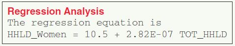
Note: Minitab shows its regression equations as instead of . Also, the notation 2.82E-07 refers to the scientific notation method of writing numbers. Often, software and calculators will present you with this type of notation, so you need to know how to read it. The number 2.82E-07 represents 2.82 times , or 0.000000282.
Question 4.157
households
59. In this exercise, we explore the regression coefficients and the regression equation.
- Find and interpret the meaning of the value for the intercept. Does it make sense?
- Would the estimate in (a) be considered extrapolation? Why or why not?
- Find and interpret the meaning of the slope coefficient as the total number of households in the state increases.
- Write the regression equation. Now state in words what the regression equation means.
- Is the correlation coefficient positive or negative? How do you know?
4.2.59
(a) 10.5. In a state with 0 households, 10.5% of the households are headed by women. Since all states have households, the value would not occur. (b) This estimate would be considered extrapolation since the value of is outside the range of -values in the data set. (c) 0.000000282. For each increase of one household, the percentage of households headed by women increases by 0.000000282. (d) (Percentage of households headed by women) = 10.5 + 0.000000282 (Total number of households). The estimated percentage of households headed by women equals 10.5 plus 0.000000282 times the total number of households. (e) Positive since the slope is positive.
Question 4.158
households
60. Estimate the increase or decrease in the percentage of households headed by women, using a sentence, for the following situations:
- Suppose State A has 1 million more households than State B.
- Suppose State C has 5 million fewer households than State D.
Question 4.159
households
61. The number of households per state ranges from about 170,000 to about 10 million.
- Estimate the percentage of households headed by women for a state with 7 million households, if appropriate.
- Estimate the percentage of households headed by women for a state with 100,000 households, if appropriate.
4.2.61
(a) 12.474% (b) is not in the range of the -values in the data set.
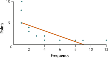
Invalid Application of Linear Regression. Use the information in the following scatterplot for Exercises 62–64. Scrabble (hasbro.com/scrabble/en_US/) is one of the most popular games in the world. We are interested in approximating the relationship between the frequency of the letter tiles in the game and their point value . The scatterplot shows the point value versus the letter frequency, along with the regression line, as plotted by Minitab.
223
Question 4.160
62. Does the relationship between frequency and points seem to be positive or negative?
Question 4.161
63. Does the relationship between frequency and points seem to be a straight-line relationship or a curved relationship?
4.2.63
Curved
Question 4.162
64. Do you think that we should use a regression line to approximate the relationship between frequency and points? If not, explain clearly what you think is wrong.
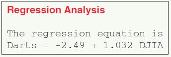
Chapter 3 Case Study (Continued). Use the following information for Exercises 65–68. Shown here is the regression equation for the linear relationship between the randomly selected Darts portfolio and the Dow Jones Industrial Average (DJIA), from the Chapter 3 Case Study. (Note: This is for the entire data set, not the small sample taken in the Exercise 39 data set.)
Question 4.163
65. In this exercise, we examine the intercept.
- Which variable is the variable and which is the variable? Work by analogy with the previous exercises.
- What is the value of the intercept?
- Interpret the meaning of this value for the intercept. Does it make sense?
- Would the estimate in (c) be considered extrapolation? Why or why not?
4.2.65
(a) Darts is the y variable and DJIA is the variable. (b) −2.49 (c) When the Dow Jones Industrial Average changes 0%, the portfolios chosen by the Darts decreases by 2.49%. Since the Dow Jones Industrial Average is based on a different set of stocks than the stock portfolio selected by the Darts, this situation makes sense. (d) The estimate in (c) would not be considered extrapolation since a value of lies within the range of the x-values of the data set.
Question 4.164
66. In this exercise, we look at the slope and the regression equation.
- Find and interpret the meaning of the value of the slope coefficient, as the DJIA increases.
- Write the regression equation. Now state in words what the regression equation means.
- Is the correlation coefficient positive or negative? How do we know?
Question 4.165
67. Estimate the increase or decrease in the net price of the Darts portfolio, using a sentence, for the following situations:
- Suppose that for Contest A the DJIA increased by 10% more than for Contest B.
- Suppose that for Contest C the DJIA decreased by 5% more than for Contest D.
4.2.67
(a) The percent change in the stocks selected by the Darts for Contest A is 1.032 (10) = 10.32% more than the percent change in the stocks selected by the Darts for Contest B. (b) The percent change in the stocks selected by the Darts for Contest C is 1.032 (5) = 5.16% less than the percent change in the stocks selected by the Darts for Contest D.
Question 4.166
68. The net change in the DJIA ranged from −13.1% to 22.5%.
- Estimate the net price change for the Darts portfolio when the DJIA is up by 22%, if appropriate.
- Estimate the net price change for the Darts portfolio when the DJIA is down by 10%, if appropriate.
- Estimate the net price change for the Darts portfolio when the DJIA is down by 22%, if appropriate.
Cell Phone Use for Internet Access, Worldwide. Would you expect that residents of richer countries tend to use their cell phones to browse the Internet more often than residents of poorer countries? The Pew Global Attitudes Project conducted a study5 of cell phone usage in countries around the world. The table shows x = the per capita gross domestic product (GDP, a measure of the wealth of the country), and y = the percentage of cell phone owners who use their cell phones to browse the Internet for a random sample of 10 countries. Use this information for Exercises 69–75.
| Nation | ||
|---|---|---|
| USA | 48,147 | 43 |
| Britain | 35,974 | 38 |
| France | 35,048 | 28 |
| Russia | 16,687 | 27 |
| Poland | 20,136 | 30 |
| Israel | 31,004 | 47 |
| China | 8,394 | 37 |
| Japan | 34,362 | 47 |
| India | 3,703 | 10 |
| Mexico | 15,121 | 18 |
Question 4.167
cellregression
69. Construct and interpret a scatterplot of the data in the table.
4.2.69
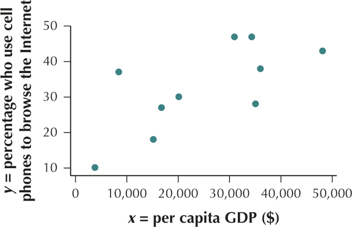
Per capita GDP ($) and percentage who use their cell phones to browse the Internet have a positive linear relationship.
Question 4.168
cellregression
70. Based on your interpretation in Exercise 69, would the value for the correlation coefficient be positive or negative?
Question 4.169
cellregression
71. Calculate the correlation coefficient .
4.2.71
Question 4.170
cellregression
72. Find the slope and intercept of the regression line. Write the regression equation in a sentence.
Question 4.171
cellregression
73. Interpret the values of the slope and the intercept. Determine whether the interpretation of the intercept represents extrapolation in this case.
4.2.73
For each increase of $1 in the country's per capita GDP the estimated percentage of cell phone users who use their cell phones to browse the Internet increases by 0.000604 percent.
The estimated percentage of cell phone users who use their cell phones to browse the Internet for a country with a per capita GDP of is 17.50%. This represents extrapolation.
Question 4.172
cellregression
74. Calculate the estimated percentage using their cell phones to browse the Internet for a nation with a per capita GDP of $48,147.
Question 4.173
cellregression
75. Identify the country with a per capita GDP of $48,147. Calculate and interpret the prediction error for this country.
4.2.75
USA. −3.58. The actual percentage of cell phone users who use their cell phones to browse the Internet for the USA of 43% lies below the estimated percentage of cell phone users who use their cell phones to browse the Internet for the USA of 46.58%.
Unidentified Flying Objects. Have you or any of your friends sighted any unidentified flying objects (UFOs)? Americans in each of the 50 states have reported seeing UFOs. Figure 30 represents a scatterplot of the number of UFO sightings versus state population, for each of the 50 states. Each dot represents a state. The straight line is a regression line, which approximates the relationship between UFO sightings and state population. As the state population increases, the number of UFO sightings also tends to increase, which is not surprising.
224
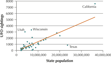
What may be surprising is that the UFOs seem to be attracted to certain states, yet avoid others. States considerably above the regression line have a larger than expected number of UFO sightings for their population size, whereas states below the line have a smaller than expected number of UFO sightings for their population size. So, there are more sightings than expected in California, Wisconsin, and Utah, given their population size, and fewer than expected in Texas. Why this might occur is open to discussion. Perhaps people in California are more likely to attribute unusual sightings to UFOs than most Americans; perhaps people in Texas are more pragmatic than most Americans. But if the sightings are valid (a big if!), it sure looks like the UFOs don’t want to mess with Texas. Refer to Figure 30 for Exercises 76–79.
Question 4.174
76. Provide a rough estimate of the following for the state of California.
- State population
- UFO sightings
Question 4.175
77. Provide a rough estimate of the following for the state of Texas.
- State population
- UFO sightings
4.2.77
(a) 23,000,000 (b) 900
Question 4.176
78. For the state of California, what is the estimated number of UFO sightings? (Hint: It’s at the point on the line directly below the dot for California.)
Question 4.177
79. For the state of Texas, what is the estimated number of UFO sightings?
4.2.79
3500
BRINGING IT ALL TOGETHER
Fuel Economy. Refer to the following table of fuel economy data for a sample of 10 vehicles for Exercises 80–84. The predictor variable is , expressed in liters; the response variable is , expressed in miles per gallon (mpg).
| Vehicle | ||
|---|---|---|
| Mini Cooper | 1.6 | 31 |
| Ford Focus | 2.0 | 28 |
| Toyota Camry | 2.5 | 26 |
| Honda Accord | 2.4 | 26 |
| Subaru Forester | 2.5 | 23 |
| Toyota Highlander | 2.7 | 22 |
| Ford Taurus | 3.5 | 20 |
| Chevrolet Equinox | 3.0 | 19 |
| Dodge Nitro | 4.0 | 17 |
| Cadillac limousine | 4.6 | 14 |
Question 4.178
enginempg
80. Exploring the Data.
- Look at the data table. As the engine size values increase, what seems to be happening to the combined mpg?
- Construct a scatterplot of the data.
- Interpret the scatterplot. Is your insight from part (a) supported?
Question 4.179
enginempg
81. What Results Do You Expect? Based on your scatterplot in Exercise 80, answer the following:
- Will the correlation coefficient be positive or negative?
- Do you expect that the correlation will be closer to −0.9 or −0.5? Why?
- Do you think that the slope will be positive or negative? Why?
4.2.81
(a) Negative; (b) 20.9; the dots lie in a pattern that is close to a straight line (c) Negative; the dots lie in a pattern that is close to a straight line with a negative slope.
Question 4.180
enginempg
82. Correlation. Do the following:
- Calculate the correlation coefficient . Does this concur with your predictions from Exercises 81(a) and 81(b)?
- Interpret the correlation between engine size and combined mpg.
Question 4.181
enginempg
83. Regression. Answer the following:
- Calculate the slope of the regression equation. Does the sign of agree with your prediction from Exercise 81(c)?
- Calculate the intercept .
- Interpret the values you calculated in parts (a) and (b), so that a nonstatistician would understand them.
4.2.83
(a) ; yes (b) = 38.41 (c) The slope of means that the combined mpg will decrease by 5.49 mpg for each 1-liter increase in engine size. The intercept of is the predicted combined mpg for an engine size of 0 liters.
Question 4.182
enginempg
84. Making Predictions. Answer the following:
- Note that the Chevrolet Equinox has an engine size of 3 liters. Predict the combined mpg for a vehicle with an engine size of 3 liters.
- Is your prediction error positive or negative? Thus, does the data value lie above or below the regression line? What does this mean?
CONSTRUCT YOUR OWN DATA SETS
Question 4.183
85. Describe two variables from real life whose regression line would have a positive slope .
- Explain why the variable depends on the variable.
- Explain why the slope is positive.
4.2.85
Answers will vary.
225
Question 4.184
86. Create a sample of five observations from each of your variables from Exercise 85, and put them into a table similar to Table 1 in Section 4.1.
- Construct a scatterplot of the variables.
- Draw a single straight line through the data points in the plot in a manner that you think best approximates the relationship between the variables.
- Using your regression line from (b), estimate the slope and the intercept .
- Write your results from (c) in the form of a regression equation.
![]() Use the Correlation and Regression applet for Exercises 87 and 88.
Use the Correlation and Regression applet for Exercises 87 and 88.
Question 4.185
87. Create a set of points, such that the slope of the regression line has the following characteristics. Note that you can drag points up or down to adjust your regression line.
- The slope is positive.
- The slope is negative.
- The slope is neither positive nor negative.
4.2.87
Answers will vary.
Question 4.186
88. Describe the relationship between the variables for each of the sets of points in the previous exercise.
WORKING WITH LARGE DATA SETS
 Chapter 4 Case Study: Measuring the Human Body. Open the data sets body_females and body_males. We will apply what we have learned in this section regarding regression analysis to some of the measurements in these data sets. Use technology for the Exercises 89–103.
Question 4.187
body_females
body_males
89. Perform a regression of weight on height for the females.
Question 4.188
body_females
body_males
90. Interpret the slope and intercept values of the regression in the previous exercise.
Question 4.189
body_females
body_males
91. Use the regression equation from Exercise 89 to estimate the weight of a female who is 63.5 inches tall.
Question 4.190
body_females
body_males
92. Find the prediction error for the first woman in the data set, with height 63.5 inches and weight 113.8 pounds.
Question 4.191
body_females
body_males
93. Estimate the weight for females with the following heights. If the estimate represents extrapolation, indicate so.
- 65 inches
- 70 inches
Question 4.192
body_females
body_males
94. Perform a regression of weight on height for the men.
Question 4.193
body_females
body_males
95. Interpret the slope and intercept values of the regression in the previous exercise.
Question 4.194
body_females
body_males
96. Use the regression equation from Exercise 94 to estimate the weight of a man who is 68.5 inches tall.
Question 4.195
body_females
body_males
97. Find the prediction error for the first male in the data set, with height 68.5 inches and weight 144.6 pounds.
Question 4.196
body_females
body_males
98. Estimate the weight for males with the following heights. If the estimate represents extrapolation, indicate so.
- 60 inches
- 65 inches
Question 4.197
body_females
body_males
99. Perform a regression of hip girth on waist girth for the women. State the regression equation in words. Note that both variables are expressed in centimeters (cm).
Question 4.198
body_females
body_males
100. Interpret the slope and intercept values of the regression of hip girth on waist girth for the women.
Question 4.199
body_females
body_males
101. Perform a regression of hip girth on waist girth, this time for the men. State the regression equation in words. Note that both variables are expressed in cm.
Question 4.200
body_females
body_males
102. Interpret the slope and intercept values of the regression of hip girth on waist girth for the males.
Question 4.201
body_females
body_males
103. Compare the similarities and differences in the regression coefficients between the women and men for the regression of hip girth on waist girth.