6.4Continuous Random Variables and the Normal Probability Distribution
OBJECTIVES By the end of this section, I will be able to …
- Identify a continuous probability distribution and state the requirements.
- Calculate probabilities for the uniform probability distribution.
- Explain the properties of the normal probability distribution.
- Find areas under the standard normal curve, given a -value.
- Compute the standard normal -value, given an area.
Sections 6.1–6.3 dealt with discrete random variables, such as the binomial random variable. Next, we turn to continuous random variables.
349
1Continuous Probability Distributions
Continuous random variables assume infinitely many possible values, with no gap between the values. For example, the height of a randomly chosen classmate of yours is a continuous random variable because it can take an infinite number of possible values.
For a given continuous random variable , we are not interested in whether equals any particular value. Instead, we are interested in whether is
- greater than a particular value, or
- less than a particular value, or
- between two particular values.
That is, we are interested in whether is located in an interval.
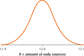
We are not interested in the probability that equals some particular value because this probability always equals zero. If this sounds crazy, then consider the following example: How much soda does a “12-ounce can” of soda actually contain? Are you sure it's 12 ounces and not 11.99999999 ounces? Or could it contain 12.00000001 ounces? In fact, the can could contain any of the infinite number of possible amounts of soda, say between 11.9 and 12.1 ounces (see Figure 19). Thus, any given amount of soda in the can is so unlikely that the probability that you will get exactly 12.00000000 ounces of soda in your 12-ounce can is essentially zero.
In contrast to the graph for a discrete distribution, the graph for a continuous probability distribution is “smooth” because it represents probability at infinitely many points along an interval.
The graph in Figure 19 is called a continuous probability distribution, defined as follows.
Continuous Probability Distribution
A continuous probability distribution is represented by a graph that indicates on the horizontal axis the range of values that the continuous random variable can take, and above which is drawn a curve, called the density curve. A continuous probability distribution must meet the following requirements.
Requirements for a Continuous Probability Distribution
- The total area under the density curve must equal 1 (this is the Law of Total Probability for Continuous Random Variables).
- The vertical height of the density curve can never be negative. That is, the density curve never goes below the horizontal axis.
2Calculating Probabilities for the Uniform Probability Distribution
To learn how to calculate probabilities for continuous random variables, we turn to the uniform probability distribution.
350
The uniform probability distribution is a continuous distribution that has constant probability from left endpoint to right endpoint . Its curve is a flat, straight line, so that the shape of the uniform distribution is a rectangle.
For example, suppose the waiting time for the campus shuttle bus follows a uniform distribution, with waiting times ranging from minutes to minutes. Then the uniform probability distribution is given in Figure 20.
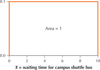
Note that the width of the rectangle in Figure 20 is . The total area under the density curve must equal 1 by the Law of Total Probability for Continuous Distributions; therefore, the height of the rectangle must equal .
So how do we represent probability for the uniform distribution, or for continuous distributions in general?
Probability for Continuous Distributions
The probability that a continuous random variable takes a value in an interval is equal to the area under the density curve above that interval.
EXAMPLE 25Uniform probability distribution
Using the uniform probability distribution in Figure 20, calculate the probability that you will wait the following amount of time for the campus shuttle bus:
- Between 2 and 4 minutes
- More than 6 minutes
- Exactly 8 minutes
Solution
We are interested in the interval between and minutes. The area above this interval forms a rectangle, shown in Figure 21. The area of this green rectangle represents the probability that is between 2 and 4 minutes. The base of the rectangle equals . The height of the rectangle equals 0.1, so we find that the area of this rectangle is
Because area represents probability, we conclude that the probability is 0.2 that you will wait between 2 and 4 minutes for the campus shuttle bus.
351
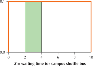 Figure 6.23: FIGURE 21 Probability that is between 2 and 4 equals the area of the green rectangle.
- The assumption that the distribution follows a uniform distribution, with waiting times ranging from minutes to minutes, means that the maximum waiting time is 10 minutes. Thus, we are interested in the interval between and . The base of this rectangle equals . Multiplied by the height of the rectangle, 0.1, the resulting . Because area represents probability, this means that the probability we will wait between 6 and 10 minutes equals 0.4.
- Here, we are not given an interval, only a single point, exactly 8 minutes. We can express this as the “interval” from 8 to 8, so that both and . Thus, the width of this “interval” is . Multiplied by the height of the rectangle, 0.1, gives us an area of . Probability equals area, so the probability that we will wait exactly 8 minutes (and not 7.99999 minutes or 8.000001 minutes) is zero. This is an example of our earlier discussion where we learned that, for continuous distributions, the probability that X exactly equals some particular value is always zero.
NOW YOU CAN DO
Exercises 11–20.
YOUR TURN #13
For the scenario in Example 25(a), find the probability that you will wait between 4 and 8 minutes for the campus shuttle.
(The solution is shown in Appendix A.)
Notice from Example 25 that the probability 0.2 equals . We generalize this as follows.
The probability that a uniform random variable with left endpoint and right endpoint takes a value in the interval [] is given by
For example, the probability that you would wait between and minutes for the campus shuttle bus is
Now, because is a continuous random variable, and . Thus, . In fact, for any continuous random variable, the inequalities ≤ and < are interchangeable, as are ≥ and >.
352
3Introduction to Normal Probability Distribution
We now turn to what is considered to be the most important probability distribution in the world: the normal probability distribution. Sometimes referred to as the bell-shaped curve (Chapter 3), the normal distribution is a continuous distribution that has been found to model accurately such phenomena as
- the amount of rainfall in Imperial Valley, California;
- the heights and weights of high-risk infants in New York City; and
- the errors in manufacturing machine bolts in a Pennsylvania factory.
Remember that, as with all probability distributions, we are dealing with a population of data values.
Similar to a discrete random variable, a continuous random variable has a mean and a standard deviation. The parameters of the normal distribution are the mean , which determines the center of the distribution on the number line, and the standard deviation , which determines the spread or shape of the distribution curve. The mean can be positive, negative, or zero; the standard deviation can never be negative.
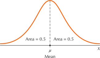
From Figure 22, we can see that the normal distribution curve is symmetric about . If you slice the curve neatly in half at the mean , the result will be two pieces that are perfect mirror images of each other, as in Figure 22.
Properties of the Normal Density Curve (Normal Curve)
- It is symmetric about, and centered at, the mean .
- The highest point occurs at because symmetry implies that the mean equals the median, which equals the mode of the distribution.
- The total area under the curve equals 1.
- Symmetry also implies that the area under the curve to the left of and the area under the curve to the right of are both equal to 0.5 (Figure 22).
- The normal distribution is defined for values of extending indefinitely in both the positive and negative directions. As moves farther from the mean, the curve approaches but never quite touches the horizontal axis.
- Values of are always found on the horizontal axis. Probabilities are represented by areas under the curve.
EXAMPLE 26Normal distribution mean and standard deviation
- Figure 23 shows two normal distributions, with different means but the same standard deviation. Which distribution has mean and which distribution has mean ?
- Figure 24 shows two normal distributions, with the same mean but different standard deviations. Which distribution has and which distribution has ?
353
Solution
- Note that the two distributions have precisely the same spread or shape because each distribution has the same standard deviation, . However, the yellow distribution is symmetric about an axis drawn at 2, and it is centered at 2. Therefore, it has mean . The green distribution is symmetrical about, and centered at . The two curves are essentially identical, with the green one shifted four units to the right.
- Because is a measure of spread, the larger the value of , the more spread out the distribution of will be. This is illustrated in Figure 24. The normal distribution with the smaller standard deviation () has a curve with a higher peak in the center and thinner “tails” than the distribution with a larger standard deviation (). Thus, the green distribution has and the yellow distribution has .
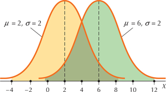 Figure 6.25: FIGURE 23 Different , same .
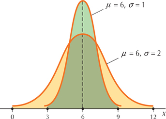 Figure 6.26: FIGURE 24 Same , different .
NOW YOU CAN DO
Exercises 21–30.
EXAMPLE 27Properties of the normal curve
A statistical study found that when nurses made home visits to pregnant teenagers to provide support services, discourage smoking, and otherwise provide care, the mean birth weight of the babies was higher for this treatment group (3285 grams) than for a control group of teenagers who were not visited (2922 grams), when the visits began before midgestation.14 The birth weights of babies are known to follow a normal distribution.15
Suppose the birth weights for the babies whose mothers were visited by the nurses (treatment group) also follow a normal distribution. Then our random variable is
The mean is grams. Assume that the standard deviation is . Graph the normal curve of .
Solution
Figure 25 shows the probability graph of . Note that the curve has the following properties:
Hint: Draw a bell-shaped curve with center at . Label the horizontal axis in increments equal to the standard deviation . Make sure the areas to the left and right of are equal.
- It is symmetric about the mean .
The highest point occurs at , which is also the median and the mode.
354
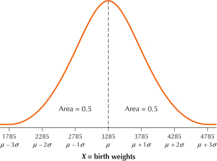 Figure 6.27: FIGURE 25 The normal curve of is symmetric about its mean .
- The total area under the curve equals 1.
- The area under the curve to the left of equals 0.5, as does the area under the curve to the right of .
NOW YOU CAN DO
Exercises 31–36.
4Finding Areas Under the Standard Normal Curve for a Given -value
Note: Understanding the techniques explained in this section will allow you to analyze a whole world of data sets, even those that are not normally distributed (see the Central Limit Theorem in the next chapter). Beyond this chapter, these techniques help you to calculate and understand -values in Chapters 9–13.
Many populations in the world are normally distributed, from test scores to student heights with different means and standard deviations. But there is one very special normal distribution called the standard normal distribution. The mean and standard deviation of the standard normal distribution make it unique.
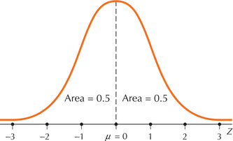
The standard normal () distribution is a normal distribution with
- mean and
- standard deviation .
Because of its importance, the standard normal random variable is always denoted as a capital . The graph of the standard normal random variable is given in Figure 26. The standard normal curve is symmetric about its mean .
355
Note: Although your table contains only values between and , there is no upper or lower limit to the values that may take. The curve essentially goes on forever in both the positive and the negative directions, always getting closer and closer to the horizontal axis but never quite touching it (there's a great plot for a love story in there somewhere).
We will discuss two methods for finding probabilities associated with , using (a) the table for finding standard normal probabilities, called the table, and (b) technology. For the table, see Table C in the Appendix. The table provides areas under the standard normal curve to the left of a specified value of Z, denoted as (see Figure 27).
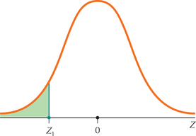
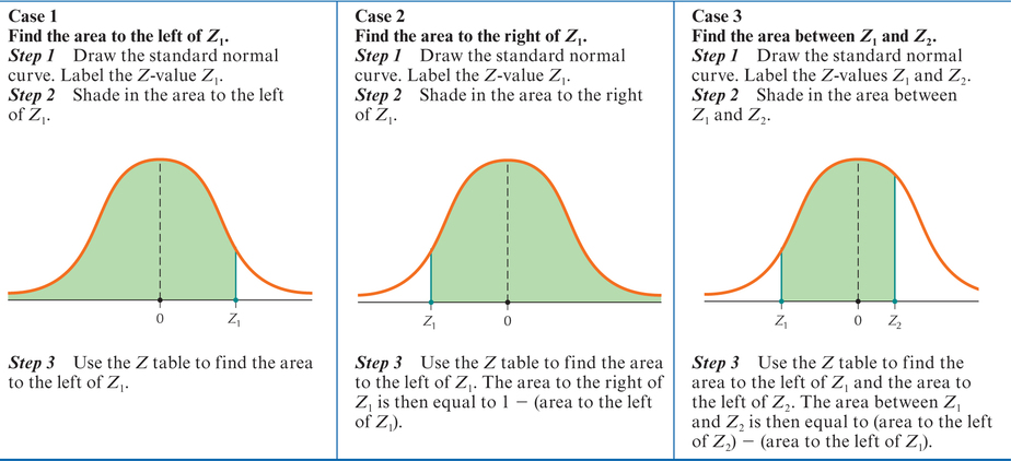
Let's get acquainted with the table (see excerpt in Figure 29 on page 356). Along the left side and across the top of the table are possible values of . These numbers, which in the table run from – 3.49 to 3.49, are the values of found on the number line when you draw a graph. Down the left are the ones and tenths digits of the -value, and across the top, is the hundredths digit. The body of the table contains areas (probabilities). These numbers, which run from 0.0002 to 0.9998, are areas under the standard normal curve that represent probabilities to the left of the specified value of . Table 8 shows the steps for finding areas under the standard normal curve, that is, for finding probabilities for specified values of .
|
356
EXAMPLE 28Case 1: Find the area to the left of a value of
Find the area to the left of .
Solution
- Step 1 First draw the standard normal curve and label .
- Step 2 Shade the area to the left of 0.57, as shown in Figure 28.
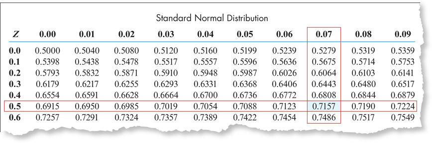
- Step 3 In the table, excerpted as Figure 29, go down the left-hand column to 0.5 and select that row. Then go across the top row (representing the hundredth's digit) to 0.07 and select that column. The quantity at the intersection of this row and column represents the area to the left of . That is, the area to the left of is 0.7157.
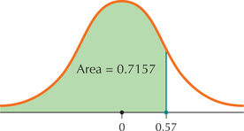 Figure 6.30: FIGURE 28 Finding the area to the left of
NOW YOU CAN DO
Exercises 37–44.
YOUR TURN #14
Find the area to the left of .
(The solution is shown in Appendix A.)
EXAMPLE 29Case 2: Find the area to the right of a value of
Find the area to the right of .
Solution
- Step 1 First draw the standard normal curve and label .
Step 2 Shade the area to the right of − 1.25, as shown in Figure 30.
357
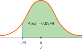 Figure 6.32: FIGURE 30 Finding the area to the right of .
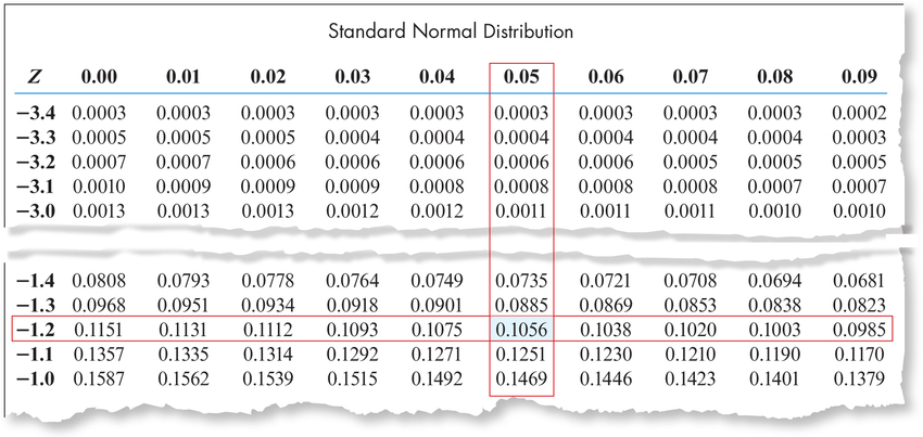
Step 3 In the table, excerpted in Figure 31, go down the left-hand column to − 1.2 and select that row. Then go across the top row to 0.05 and select that column. The area to the left of is therefore 0.1056. From Case 2 in Table 8, the area to the right of −1.25 is then
 Remember that, although values of can be negative, probabilities (or areas) can never be negative.
NOW YOU CAN DO
Exercises 45–48.
YOUR TURN #15
Find the area to the right of .
(The solution is shown in Appendix A.)
Developing Your Statistical Sense
Checking That Your Answer Makes Sense
As you are finding probabilities for values of , you should always be checking to see that your answer makes sense. For instance, in Example 29, what if we had added the table area to 1 instead of subtracted the table area from 1? We would know that this answer is incorrect because the resulting probability would then have exceeded 1, and no probability can ever exceed 1.
358
EXAMPLE 30Case 3: Find the area between two (checking the accuracy of the Empirical Rule)
Recall that the Empirical Rule (page 135 of Chapter 3) states that about 68% of the area under the curve lies within 1 standard deviation of the mean, that is, between and . Check this result for the standard normal distribution by using the table.
Solution
For the standard normal random variable and , so that and . Thus, using Case 3, we have and .
- Step 1 Draw the standard normal curve. Label the and .
- Step 2 Shade the area between − 1 and 1, as shown in Figure 32a.
- Step 3 Find the area to the left of and the area to the left of . The table gives these areas as follows: area to the left of is 0.1587, and area to the left of is 0.8413. We subtract the smaller area from the larger to give us the area between − 1 and 1, as shown in Figures 32a–32c.
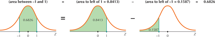 Figure 6.34: FIGURE 32a To get the area we are looking for…FIGURE 32b Find the area to the left of 1…FIGURE 32c And subtract the area to the left of −1.
NOW YOU CAN DO
Exercises 49–58.
Thus, the area under the curve within 1 standard deviation of the mean equals 0.6826. The Empirical Rule does very well for an approximation, missing the actual area by only 0.0026. Checking the accuracy of the Empirical Rule for other values of is left as an exercise.
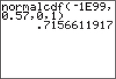
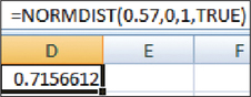
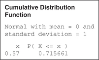
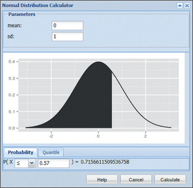
EXAMPLE 31Using technology to find the area under a standard normal curve
In Example 28, we found the area under the standard normal curve to the left of to be 0.7157. Confirm this result using technology.
Solution
We follow the instructions in the Step-by-Step Technology Guide at the end of Section 6.5 (page 380). Figures 33, 34, 35, and 36 show the results from TI-83/84, Excel, Minitab, and CrunchIt!, respectively.
The word “cumulative” in the Minitab output means “less than or equal to.” Each of these results provides the area under the standard normal curve for values of that are less than or equal to 0.57. Each technology rounds to a different number of decimal places.
![]() The Normal Density Curve applet allows you to find areas associated with various values of
The Normal Density Curve applet allows you to find areas associated with various values of
359
Note that the areas we have been finding in this section may also be expressed as probabilities. For continuous distributions, probabilities are represented by areas under the curve above an interval. Specifically, for the standard normal distribution, probability is represented as the area above an interval under the standard normal curve. For instance, in Example 28, we found that the area under the standard normal curve to the left of is 0.7157. This may be re-expressed as follows:
“The probability that is less than 0.57 is 0.7157”
or
EXAMPLE 32Expressing areas under the standard normal curve as probabilities
Re-express the following areas as probabilities:
- In Example 29, we found the area under the standard normal curve to the right of to be 0.8944.
- In Example 30, we found the area under the standard normal curve between and to be 0.6826.
Solution
- The probability that is greater than − 1.25 is 0.8944. That is, .
- The probability that is between − 1 and 1 is 0.6826. That is, .
NOW YOU CAN DO
Exercises 59–70.
5Finding Standard Normal -values for a Given Area
In previous examples, we were given a -value and asked to find an area or probability. What if we turned this around, so that we are given an area, and asked to find its associated -value? We may call these “backward” problems because we would need to use the table in reverse (unless we are using technology to solve the problem). Let's check out an example.
360
EXAMPLE 33Finding the -value with given area to its left
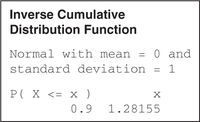
Recall that the th percentile is the value in the data set such that percent of the data values fall at or below that value. Thus, represents the 90th percentile of the distribution because it is greater than 90% of -values.
Find the -value with area 0.90 to its left.
Solution
- Step 1 Draw the standard normal curve. Label the .
- Step 2 Shade the area to the left of . Remember that we are given an area and are looking for a value of . Label the area to the left of with the given area (0.90), as shown in Figure 37.
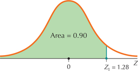 Figure 6.39: FIGURE 37 is the value of with area 0.90 to the left of it.
 - Step 3 Look for 0.90 on the inside of the table (that is, in the body of the table), because the values inside the table represent areas. Because there is no 0.90 inside the table, by convention we take the area that is closest to 0.90, which is 0.8997. Next is the trick of the backward problems and the reason for that name. Move from 0.8997 to the left until you reach 1.2 in the first column, and then move up from 0.8997 until you get to 0.08 (see Figure 38). Putting these values together, we get .
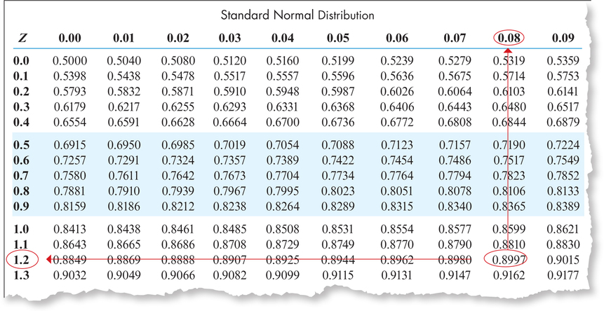 Figure 6.40: FIGURE 38 Using the table to find a value of for a given area.
NOW YOU CAN DO
Exercises 71–78.
YOUR TURN #16
Find the -value with area 0.975 to its left.
(The solution is shown in Appendix A.)
361
EXAMPLE 34Find the -value with given area to its right
Find the standard normal -value that has area 0.03 to the right of it.
Solution
- Step 1 Draw the standard normal curve. Label the . Shade the area to the right of it with the given area, as shown in Figure 39.
Step 2 The table contains areas to the left of values of , so we must find the area to the left of the specific value , as follows:
So the area to the left of is .
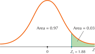 Figure 6.41: FIGURE 39 has an area 0.03 to the right of it.
- Step 3 Look up 0.97 on the inside of the table. The closest area is 0.9699. Move from 0.9699 to the left until you reach 1.8, and then move up from 0.9699 until you get to 0.08 (see Figure 40). Putting these values together, we get . In other words, the -value with area 0.03 to its right is .
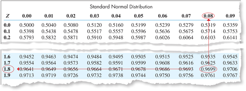 Figure 6.42: FIGURE 40 Using the table to find a value of for a given area.
NOW YOU CAN DO
Exercises 79–86.
YOUR TURN #17
Find the -value with area 0.975 to its right. (The solution is shown in Appendix A.)
When we learn statistical inference in later chapters, we will need to identify which divide the middle 90%, 95%, or 99% of the area under the standard normal curve from the tail area.
362
EXAMPLE 35Find the values of that mark the boundaries of the middle 95% of the area
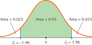
Find the two values of that mark the boundaries of the middle 95% of the area under the standard normal curve.
Solution
Note: Is it a coincidence that the two values of that determine the middle 95% of the area under the standard normal curve are 1.96 and 21.96? Not at all. The standard normal curve is symmetric about the mean 0, so the values −1.96 and 1.96 that form the boundaries of the middle 95% must be equidistant from zero.
- Step 1 Draw the standard normal curve, showing the desired middle area (95%) with boundaries labeled as and , as shown in Figure 41. By symmetry, there is in each tail.
- Step 2 Look up 0.025 on the inside of the table. Find by moving to the left and up from 0.025 in the table, giving us .
- Step 3 The area in the right tail is also 0.025, so the area to the left of is . Looking up 0.975 in the table gives us .
NOW YOU CAN DO
Exercises 87–90.
Thus, the two that mark the boundaries of the middle 95% of the area under the standard normal curve are − 1.96 and 1.96. This is a more precise result, which states that about 95% lies between – 2 and 2.
YOUR TURN #18
Find the two values of that mark the boundaries of the middle 90% of the area under the standard normal curve.
(The solution is shown in Appendix A.)
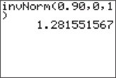
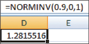
EXAMPLE 36Using technology to find values of , given an area
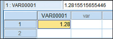
In Example 33, we found that the value of with area 0.90 to its left is . Con-frm this result with technology.
Solution
We follow the instructions in the Step-by-Step Technology Guide at the end of Section 6.5 (page 380). Figures 42, 43, 44, and 45 show the results from TI-83/84, Excel, Minitab, and SPSS, respectively. Note that technology usually provides a more precise solution than the table.
363