6.1Discrete Random Variables
310
OBJECTIVES By the end of this section, I will be able to …
- Identify random variables.
- Explain what a discrete probability distribution is and construct probability distribution tables and graphs.
- Calculate the mean, variance, and standard deviation of a discrete random variable.
1Random Variables
In Chapter 5, we calculated the probabilities of outcomes from experiments. If the experiment is tossing a fair coin twice, the outcomes are , , , and . The probability of observing exactly one head in two tosses is the probability of the event . Because the outcomes were equally likely, we used the classical method of assigning probability. The probability of is , where is the sample space.
In this chapter, we develop a different approach that analyzes probability problems more efficiently. Recall from Chapter 1 that a variable is a characteristic that can assume different values. Suppose we define a variable X = number of heads observed when two fair coins are tossed. In this experiment we may observe zero heads, one head, or two heads, so that the possible values of are 0, 1, and 2. Clearly, before we conduct our experiment, we do not know how many heads we will observe. Thus, randomness plays a role in the value of the variable , and so we call a random variable.
A random variable is a variable that takes on quantitative values representing the results of a probability experiment, and thus its values are determined by chance. We denote random variables using capital letters such as , , or .
In Chapter 5 (page 246), we found that the probability of observing exactly X = one head was 0.5. We denote this probability using the notation
Similarly, the probability of observing zero heads is , and the probability of two heads is .
Developing Your Statistical Sense
Random Variables Must Be Random!
The role of chance in the definition of a random variable is crucial. For example, is your age a random variable? If we are just talking about you and no one else, and we know your age, then there is no chance involved. In that case, your age is not a random variable. On the other hand, what if we select students at random by picking names from a hat? Then the age of the person drawn is a random variable because its value depends at least partly on chance (on which name is drawn at random).
Let's start with an example aimed at helping you move from the language of probability (experiments and outcomes) to the language of random variables.
311
EXAMPLE 1Notation for random variables
Suppose our experiment is to toss a single fair die, and we are interested in the number rolled. We define our random variable to be the outcome of a single die roll.
- Why is the variable a random variable?
- What are the possible values that the random variable can take?
- What is the notation used for rolling a 5?
- Use random variable notation to express the probability of rolling a 5.
Solution
- We don't know the value of before we toss the die, which introduces an element of chance into the experiment, thereby making a random variable.
- The possible values for are 1, 2, 3, 4, 5, and 6.
- When a 5 is rolled, then equals the outcome 5, and we write .
- Recall from Section 5.1 that the probability of rolling a 5 for a fair die is 1/6. In random variable notation, we denote this as .
There are two main types of random variables: discrete random variables and continuous random variables. The difference between the two types relates to the possible values that each type of random variable can assume.
Discrete random variables usually need to be counted, such as 1, 2, 3, and so forth. Continuous random variables usually need to be measured, not counted, such as measuring the amount of gasoline purchased.
Discrete and continuous random variables
- A discrete random variable can take either a finite or a countable number of values. These values may be written as a list of numbers, so each value can be graphed as a separate point on a number line, with space between each point. (See Figure 1a.)
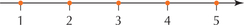 Figure 6.1: FIGURE 1a Discrete random variable.
 - A continuous random variable can take uncountably infinite different values. Because of this, the values of a continuous random variable form an interval on the number line. (See Figure 1b.)
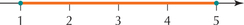 Figure 6.2: FIGURE 1b Continuous random variable.
Examples of discrete random variables include the number of children a randomly selected person has and the number of times a randomly chosen student has been pulled over for speeding on the interstate. Continuous random variables often need to be measured, not counted. For example, the temperature in Atlanta, Georgia, at noon today may be reported as 77 degrees, but this value represents actual temperatures that may lie anywhere between 76.5 degrees and 77.5 degrees.
EXAMPLE 2Identifying discrete and continuous random variables
For the following random variables, (i) determine whether they are discrete or continuous, and (ii) indicate the possible values they can take:
- The number of automobiles owned by a family
- The width of your desk in this classroom
- The number of games played in the next World Series
- The weight of model year 2015 SUVs
312
Solution
- The possible number of automobiles owned by a family is finite and may be written as a list of numbers, so it represents a discrete random variable. The possible values are .
- Width is something that must be measured, not counted. Width can take infinitely many different possible values, with these values forming an interval on the number line. Thus, the width of your desk is a continuous random variable. The possible values might be .
- The number of games played in the next World Series can be counted and thus represents a discrete random variable. The possible values are finite and may be written as a list of numbers: .
- The weight of model year 2015 SUVs must be measured, not counted, and thus represents a continuous random variable. Weight can take infinitely many different possible values, with these values forming an interval on the number line: .
NOW YOU CAN DO
Exercises 7–16.
YOUR TURN #1
For the following random variables, (i) determine whether they are discrete or continuous, and (ii) indicate the possible values they can take:
- Your best friend's height
- The number of cats you own
(The solutions are shown in Appendix A.)
We will return to continuous random variables in Section 6.4. Sections 6.1, 6.2, and 6.3 concentrate on discrete random variables.
2Discrete Probability Distributions
For every random variable, there is a probability distribution that allows us to view all possible values of the random variable at a glance. Discrete probability distributions show the probabilities associated with the various values that the discrete random variable can take.
A probability distribution of a discrete random variable provides all the possible values that the random variable can assume, together with the probability associated with each value. The probability distribution can take the form of a table, graph, or formula. Probability distributions describe populations, not samples.
When constructing the tabular form of a probability distribution of a discrete random variable, create a table with two rows:
- The top row will contain all the possible values of .
- The bottom row will contain the probability associated with each value of .
EXAMPLE 3Probability distribution table
Construct the probability distribution table of the number of heads observed when tossing a fair coin twice.
Solution
The probability distribution table given in Table 1 uses the probabilities we found on page 246.
313
| 0 | 1 | 2 | |
|---|---|---|---|
| 1/4 | 1/2 | 1/4 |
The probabilities in Table 1 were assigned using the classical method, because we assumed that tossing a fair coin would result in equally likely outcomes.
NOW YOU CAN DO
Exercises 17a–24a.
Note that the probabilities in the bottom row of Table 1 add up to 1. Also, note that because each value in the bottom row is a probability, each value must be between 0 and 1, inclusive, that is, . We can generalize this as follows.
Rules for a Discrete probability Distribution
- The sum of the probabilities of all the possible values of a discrete random variable must equal 1. That is, .
- The probability of each value of must be between 0 and 1, inclusive. That is, .
This first rule derives from the Law of Total Probability from Section 5.1 (page 241).
EXAMPLE 4Recognizing valid discrete probability distributions
Identify which of the following is a valid discrete probability distribution.
1 10 100 1000 0.2 0.4 0.3 0.2 −10 0 10 20 0.5 0.3 0.4 −0.2 Red Green Blue Yellow 0.1 0.3 0.4 0.2 −5 0 5 10 0.1 0.3 0.4 0.2
Solution
- This is not a valid probability distribution because the probabilities add up to 1.1, which is greater than 1.
- This is not a valid probability distribution because is negative.
- This is not a valid probability distribution for a discrete random variable because the values of are not quantitative.
- This is a valid probability distribution because the probabilities sum to 1, and each probability takes a value between 0 and 1.
NOW YOU CAN DO
Exercises 25–28.
314
YOUR TURN #2
Identify whether the following is a valid discrete probability distribution.
| −4 | −2 | 0 | 2 | |
|---|---|---|---|---|
| 0.25 | 0.30 | 0.30 | 0.20 |
(The solution is shown in Appendix A.)
Probability distributions can also take the form of a probability distribution graph.
EXAMPLE 5Discrete probability distribution as a graph
The number of points a soccer team gets for a game is a random variable because it is not certain, before the game, how many points the team will get.

In Major League Soccer (MLS), teams are awarded 3 points in the standings for a win, 1 point for a tie, and 0 points for a loss. In the 34-game 2013 MLS season, the New York Red Bulls had 17 wins, 9 losses, and 8 ties.
- Construct a probability distribution table of the number of points per game, based on the team's performance during the 2013 MLS season.
- Construct a probability distribution graph of the number of points per game.
Solution
The probabilities in Table 2 were assigned to the random variable using the relative frequency (empirical) method.
- Let . Then the probability distribution table is given in Table 2.Table 6.7: Table 2Probability distribution table of points awarded for New York Red Bulls
0 1 3 - The probability distribution graph is given in Figure 2.
- The horizontal axis is the usual x axis (the number line), and it shows all the possible values that the random variable can take, such as . The horizontal axis gives the same information as the top row of the table.
- The vertical axis represents probability, and is the information in the bottom row in the table. A vertical bar is drawn at each value of , with the height representing the probability of that value of . For example, the bar of probability at goes up to 0.26 and represents the probability that the New York Red Bulls will lose a game.
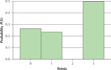 Figure 6.3: FIGURE 2 Probability distribution graph of points awarded for New York Red Bulls.
Given a graph of a probability distribution, you should know how to construct the probability distribution table, and vice versa.
NOW YOU CAN DO
Exercises 17b–24b.
315
YOUR TURN #3
Construct a probability distribution graph of the number of heads observed in Table 1 on page 313.
(The solution is shown in Appendix A.)
We may use probability distributions to calculate probabilities for multiple values of . In discrete probability distributions, the outcomes are always mutually exclusive. For example, it is not possible to observe both zero heads and two heads when tossing two fair coins. Thus, we always use the Addition Rule for Mutually Exclusive Events to find the probability of two or more outcomes for a discrete random variable. For example, .
EXAMPLE 6Calculating probabilities for multiple values of
Use the probability distribution from Example 5 to find the following probabilities:
- Probability that the New York Red Bulls are awarded either 0 or 3 points in a game
- Probability that the New York Red Bulls are awarded both 0 and 3 points in a game
- Probability that the New York Red Bulls are awarded at least 1 point in a game
- Probability that the New York Red Bulls are awarded at most 1 point in a game
Solution
- . For a randomly selected game, the probability that the Red Bulls either lose the game or win the game is 0.76.
- The outcomes and are mutually exclusive. Therefore, .
- The phrase at least means “that many or more.” Thus, we need to find: .
- The phrase at most means “that many or fewer.” Thus, .
NOW YOU CAN DO
Exercises 29–44.
YOUR TURN #4
For the situation in Example 6, what is the probability that the New York Red Bulls are awarded the following number of points in a game?
- Either 1 point or 3 points
- Both 1 point and 3 points
- At most 3 points
- At least 3 points
(The solutions are shown in Appendix A.)
3Mean and variability of a Discrete random variable
Just as we can compute the mean and standard deviation of quantitative data, we can calculate the mean and standard deviation of a random variable .
The mean of a discrete random variable represents the mean result when the experiment is repeated an indefinitely large number of times.
316
Finding the Mean of a Discrete random variable
The mean of a discrete random variable is found as follows:
- Multiply each possible value of by its probability.
- Add the resulting products.
This procedure is denoted as
EXAMPLE 7Calculating the mean of a discrete probability distribution
Note: These 10 friends constitute a population, not a sample, so the mean is , not
Carla has 10 friends in school. She took a census of all 10 friends, asking each how many credits they had registered for that semester. Five of her friends were taking 15 credits, with one each taking 12, 13, 14, 16, and 20 credits. The relative frequency distribution is shown in Table 3.
| Credits | Frequency | Relative frequency |
|---|---|---|
| 12 | 1 | 0.1 |
| 13 | 1 | 0.1 |
| 14 | 1 | 0.1 |
| 15 | 5 | 0.5 |
| 16 | 1 | 0.1 |
| 20 | 1 | 0.1 |
- Construct the probability distribution table for .
- Calculate the mean number of credits taken.
Solution
- Our random variable is . We use the relative frequencies from Table 3 to assign probabilities to the various values of . The resulting probability distribution table is shown in the first two columns of Table 4.
To find the mean , we first need to multiply each possible outcome (value of ) by its probability . This is shown in the right-hand column in Table 4. We multiply the value by its probability , the value by its probability , and so on. Then we add these five products to find the mean:
Table 6.9: Table 4Probability distribution table of12 0.1 13 0.1 14 0.1 15 0.5 16 0.1 20 0.1 Total 1.0
317
The mean number of credits taken by Carla's friends is 15.
NOW YOU CAN DO
Exercises 45a–52a.
YOUR TURN #5
Refer to Table 1 on page 313. Calculate the mean number of heads.
(The solution is shown in Appendix A.)
What Does This Number Mean?
What does it mean to say that is the mean of the random variable First of all, the mean of the random variable is definitely not the same as the mean of a sample of Carla's friends, which is a sample mean. For example, suppose that a sample of 4 of Carla's 10 friends were taking the following number of credits: 15, 14, 13, 12. The mean of this sample of four friends is . However, if we were to consider an infinite number of friends, then the mean of this very large sample would converge to . So the mean of a discrete random variable is interpreted as the mean of the results from the population of all possible repetitions of the experiment, which is why we denote the mean of a random variable as .
Note: The population mean does not need to equal any values of , nor does it need to be an integer.
Developing Your Statistical Sense
Why Does This Formula Work?
The formula for the mean of a discrete random variable works because it is a special case of the weighted mean (page 149 of Chapter 3). Of the population of 10 friends, 1 was taking 12 credits. Thus, the first weight is . Similarly, , and . Thus, the population weighted mean is
Dividing through and rearranging terms give us
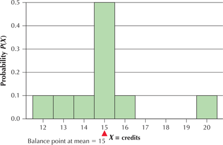
We may also interpret the mean as the balance point of the distribution.
EXAMPLE 8Mean as balance point of the distribution
Graph the probability distribution of the random variable , and insert a pivot (a balance point) at the value of the mean, .
Solution
The probability distribution graph of is given in Figure 3. Note that the distribution is balanced at the point .
318
YOUR TURN #6
Refer to Table 1 on page 313. Graph the probability distribution of the random variable , and insert a pivot (a balance point) at the value of the mean, .
(The solution is shown in Appendix A.)
In certain situations, we may need to identify the most likely value of the random variable .
EXAMPLE 9Identifying the most likely value of a discrete random variable
If one of the friends represented in the table in Example 7 is chosen at random, what is the most likely number of credits taken by that friend?
Solution
The largest probability in the probability table is , and the tallest bar in the probability graph (Figure 3) is for , so 15 is the most likely number of credits.
NOW YOU CAN DO
Exercises 45b–52b.
YOUR TURN #7
Refer to Table 1 on page 313. Identify the most likely number of heads when a fair coin is tossed twice.
(The solution is shown in Appendix A.)
Note: In Example 9, the most likely number of credits equals the mean, but this is not typical. Very often, the most likely value of a random variable is not equal to the mean.
The mean of a random variable is also called the expected value or the expectation of the random variable . It does not necessarily follow that the expected value of is the most likely value of . However, the expected value of (that is, the mean ) is often a good indication of the center of the distribution of the random variable.
The expected value, or expectation, of a random variable is the mean of . It is denoted as . This definition holds for both discrete and continuous random variables.
EXAMPLE 10Expected value of a discrete random variable
Find the expected value of the following discrete random variables:
- in Example 3
- awarded in Example 5
- in Example 7
319
Solution
Using the probabilities in Table 1, we have
The expected number of heads is 1.
Using Table 2, we have
The expected number of points is 1.74.
- From Example 7, . The expected number of credits is 15.
NOW YOU CAN DO
Exercises 45c–52c.
Note from Example 10(b) that the mean or expected value of a random variable need not be a particular value of . Instead, it represents the mean of a very large number of repetitions of the experiment.
Variability of a Discrete Random Variable
Because a discrete random variable takes on quantitative values, we use the variance or standard deviation of a random variable to help us determine whether a particular value of that random variable is unusual. Just as a random variable has a mean (), which is a measure of center, so a random variable also has a standard deviation () and variance (), which are measures of spread.
Variance and standard Deviation of a Discrete Random Variable
Notice that these formulas include as one of the terms, so that you must first find the mean of the discrete random variable before you find the variance (or standard deviation). Recall from Chapter 3 that the standard deviation is simply the square root of the variance.
EXAMPLE 11Calculating the variance and standard deviation of a discrete random variable
The probability distribution for the number of credits is repeated here as Table 5. In Example 7, we calculated the mean number of credits as . Calculate the variance and standard deviation.
| 12 | 0.1 |
| 13 | 0.1 |
| 14 | 0.1 |
| 15 | 0.5 |
| 16 | 0.1 |
| 20 | 0.1 |
Solution
Refer to Table 6. The first two columns correspond to the probability distribution of . The third column represents the calculations needed to find . Summing the values in the rightmost column provides the variance . Taking the square root of the variance gives us the standard deviation credits.
320
credits
| 12 | 0.1 | |
| 13 | 0.1 | |
| 14 | 0.1 | |
| 15 | 0.5 | |
| 16 | 0.1 | |
| 20 | 0.1 | |
NOW YOU CAN DO
Exercises 53a,b–60a,b.
Now that we have calculated the standard deviation , we may use it along with the mean to determine whether values of are outliers or moderately unusual, using the -score method.
EXAMPLE 12-score method for determining an unusual value
- Using the information from Example 11, determine whether is an unusual number of credits to take this semester.
- Construct a probability distribution graph of , illustrating how credits is moderately unusual.
Solution
Recall from Section 3.4 (page 159) that a data value with a -score between 2 and 3 may be considered moderately unusual. The -score for credits is
Thus, among Carla's friends, it would be considered moderately unusual to take 20 credits this semester.
- Figure 4 shows the probability distribution graph of . The mean is indicated, along with the distances , , .
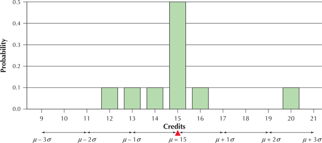 Figure 6.5: FIGURE 4 credits is moderately unusual because it lies standard deviations above the mean.
NOW YOU CAN DO
Exercises 53c–60c.
321
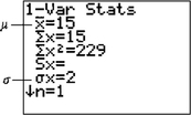
EXAMPLE 13Compute the mean and standard deviation of a discrete random variable using technology
Compute the mean and standard deviation of the probability distribution given in Example 11 using the TI-83/84 graphing calculator.
Solution
We use the instructions provided in the following Step-by-Step Technology Guide. The results are shown in Figure 5. Be careful! The calculator indicates that the mean is . It is not but .