Section 8.1 Exercises
CLARIFYING THE CONCEPTS
Question 8.1
1. Explain why a point estimate, together with a margin of error, is more likely to capture the value of a population parameter than a point estimate alone. (p. 429)
8.1.1
A range of values is more likely to contain than a point estimate is to be exactly equal to μ. We have no measure of confidence that our point estimate is close to μ. A confidence level for a confidence interval means that if we take sample after sample for a very long time, then in the long run, the percent of intervals that will contain the population mean will equal the confidence level.
Question 8.2
2. What are two ways of presenting a confidence interval? (p. 429)
Question 8.3
3. Suppose that a 95% confidence interval for the population mean football score is (15, 25). Interpret this confidence interval. (p. 433)
8.1.3
We are 95% confident that the population mean football score lies between 15 and 25.
Question 8.4
4. True or false: It is the confidence interval that is random, not the population mean . (p. 435)
Question 8.5
5. Let represent the margin of error. Explain what the “±” notation means in . (p. 433)
8.1.5
is shorthand for writing the two values and is shorthand notation for writing two numbers.
Question 8.6
6. What is the difference between confidence interval and confidence level? (p. 430)
Question 8.7
7. Assume that the confidence level increases.
- What happens to the value of ? (p. 432)
- Explain why this happens. Draw a sketch to help you. (p. 432)
8.1.7
(a) increases. (b) Since the confidence level is , as the confidence level increases, increases. Thus and will decrease. Since is the area underneath the standard normal curve to the right of , a decrease in will result in an increase in .
Question 8.8
8. Suppose your supervisor wants to (a) increase the confidence level from 95% to 99% and (b) keep the width of the confidence interval small. What is the only way to accomplish this? (p. 439)
Question 8.9
9. What happens to the required sample size for estimating the population mean as the confidence level is increased? Decreased? (p. 440)
8.1.9
Increases, Decreases
Question 8.10
10. What happens to the required sample size for estimating the population mean as the margin of error is increased? Decreased? (p. 441)
PRACTICING THE TECHNIQUES
 CHECK IT OUT!
| To do | Check out | Topic |
|---|---|---|
| Exercises 11–14 | Example 1 | Calculating a point estimate |
| Exercises 15–20 | Example 2 | Determining whether the interval for may be used |
| Exercises 21–26 | Example 3 | Finding the value of |
| Exercises 27–30 | Example 4 | Constructing a confidence interval for the mean of a normal population |
| Exercises 31–34 | Example 5 | Constructing a interval for the population mean for a large sample size |
| Exercises 35–42 | Example 7 | Finding and interpreting the margin of error |
| Exercises 43–46 | Example 10 | Finding the margin of error, given the lower and upper bounds |
| Exercises 47–54 | Example 11 | Sample size considerations |
For the data sets shown in Exercises 11–14, calculate the point estimate of the population mean .
444
Question 8.11
11.
| 4 | 5 | 3 | 5 | 3 |
8.1.11
4
Question 8.12
12.
| 18 | 14 | 16 | 14 | 18 |
Question 8.13
13.
| 10 | 16 | 13 | 16 | 10 |
8.1.13
13
Question 8.14
14.
| 100 | 108 | 104 | 100 | 108 |
For Exercises 15–20, random samples are drawn. Indicate whether or not we can use the confidence interval for .
Question 8.15
15. The sample size is large and is unknown.
8.1.15
No
Question 8.16
16. The original population is normal and is known.
Question 8.17
17. The sample size is large and is known.
8.1.17
Yes
Question 8.18
18. The sample size is small , the original population is normal, and is known.
Question 8.19
19. The sample size is large , the original population is not normal, and is known.
8.1.19
Yes
Question 8.20
20. The original population is not normal, and is not known.
For Exercises 21–26, find the value of .
Question 8.21
21. Confidence level = 99%
8.1.21
Question 8.22
22.
Question 8.23
23. Confidence level = 95%
8.1.23
Question 8.24
24.
Question 8.25
25. Confidence level = 90%
8.1.25
Question 8.26
26.
For Exercises 27–34, answer the following questions:
- Calculate .
- Find for a confidence interval for with 95% confidence.
- Construct and interpret a 95% confidence interval for .
Question 8.27
27. A random sample of with sample mean is drawn from a normal population in which .
8.1.27
(a) 2.5 (b) 1.96 (c) (70.1, 79.9). We are 95% confident that the population mean lies between 70.1 and 79.9.
Question 8.28
28. A random sample of with sample mean is drawn from a normal population in which .
Question 8.29
29. A random sample of with sample mean is drawn from a normal population in which .
8.1.29
(a) 2.6667 (b) 1.96 (c) (14.7733, 25.2267). We are 95% confident that the population mean lies between 14.7733 and 25.2267.
Question 8.30
30. A random sample of with sample mean is drawn from a normal population in which .
Question 8.31
31. A random sample of with sample mean is drawn from a population in which .
8.1.31
(a) 1 (b) 1.96 (c) (18.04, 21.96). We are 95% confident that the population mean lies between 18.04 and 21.96.
Question 8.32
32. A random sample of with sample mean is drawn from a population in which .
Question 8.33
33. A random sample of with sample mean is drawn from a population in which .
8.1.33
(a) 0.1 (b) 1.96 (c) (−5.196, −4.804). We are 95% confident that the population mean lies between −5.196 and −4.804.
Question 8.34
34. A random sample of with sample mean is drawn from a population in which .
For Exercises 35–42, do the following:
- Compute the margin of error for the confidence interval constructed in the indicated exercise.
- Interpret this value for the margin of error.
Question 8.35
35. Confidence interval from Exercise 27
8.1.35
(a) 4.9 (b) We can estimate the population mean to within 4.9 with 95% confidence.
Question 8.36
36. Confidence interval from Exercise 28
Question 8.37
37. Confidence interval from Exercise 29
8.1.37
(a) 5.2267 (b) We can estimate the population mean to within 5.2267 with 95% confidence.
Question 8.38
38. Confidence interval from Exercise 30
Question 8.39
39. Confidence interval from Exercise 31
8.1.39
(a) 1.96 (b) We can estimate the population mean to within 1.96 with 95% confidence.
Question 8.40
40. Confidence interval from Exercise 32
Question 8.41
41. Confidence interval from Exercise 33
8.1.41
(a) 0.196 (b) We can estimate the population mean to within 0.196 with 95% confidence.
Question 8.42
42. Confidence interval from Exercise 34
For Exercises 43–46, software output from a confidence interval for is provided. For each, examine the indicated software output, and do the following:
- Report the confidence interval in the form “(lower bound, upper bound).”
- Interpret the confidence interval.
- Calculate the margin of error for the confidence interval.
- Interpret the margin of error.
Question 8.43
43. TI-83/84 output, where represents the population mean intelligence test score. Confidence level = 95%.
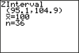
8.1.43
(a) (95.1, 104.9) (b) We are 95% confident that the population mean lies between 95.1 and 104.9. (c) 4.9 (d) We can estimate the population mean to within 4.9 with 95% confidence.
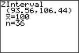
Question 8.44
44. TI-83/84 output, where represents the population mean intelligence test score. Confidence level = 99%.
Question 8.45
45. Minitab output, where represents the population mean GPA of college freshmen.
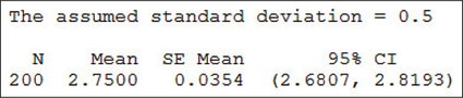
8.1.45
(a) (2.6807, 2.8193) (b) We are 95% confident that the population mean lies between 2.6807 and 2.8193. (c) 0.0693 (d) We can estimate the population mean to within 0.0693 with 95% confidence.
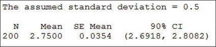
Question 8.46
46. Minitab output, where represents the population mean GPA of college freshmen.
Suppose we are estimating . For Exercises 47–49, find the required sample size.
Question 8.47
47. , confidence level 95%, margin of error 32
8.1.47
1
Question 8.48
48. , confidence level 95%, margin of error 16
Question 8.49
49. , confidence level 95%, margin of error 8
8.1.49
7
Question 8.50
50. What happens to the required sample size when the margin of error is halved and and the confidence level stay the same?
445
Suppose we are estimating . For Exercises 51–53, find the required sample size.
Question 8.51
51. , confidence level 90%, margin of error 10
8.1.51
3
Question 8.52
52. , confidence level 95%, margin of error 10
Question 8.53
53. , confidence level 99%, margin of error 10
8.1.53
7
Question 8.54
54. What happens to the required sample size when the confidence level increases and the margin of error and stay the same?
APPLYING THE CONCEPTS
Question 8.55
55. Increasing Confidence. A random sample of is drawn from a normal population in which . The sample mean is . For (a)-(c), construct and interpret confidence intervals for with the indicated confidence levels. Then answer the question in (d).
- 90%
- 95%
- 99%
- What can you conclude about the width of the interval as the confidence level increases?
8.1.55
(a) (9.342, 10.658) (b) (9.216, 10.784) (c) (8.9696, 11.0304) (d) It increases.
Question 8.56
56. Decreasing Confidence. A random sample of is drawn from a population in which . The sample mean is . For parts (a)-(c), construct and interpret confidence intervals for with the indicated confidence levels. Then answer the question in (d).
- 99%
- 95%
- 90%
- What can you conclude about the width of the interval as the confidence level decreases?
For each of Exercises 57–60, do the following:
- Find the point estimate of the population mean.
- Calculate .
- Find for a confidence interval for the indicated confidence level.
- Confirm that the conditions for constructing a interval are met.
- Construct and interpret a confidence interval with the indicated confidence level for the population mean.
Question 8.57
57. Consumption of Carbonated Beverages. The U.S. Department of Agriculture reports that the mean American consumption of carbonated beverages per year is greater than 52 gallons. A random sample of 30 Americans yielded a sample mean of 69 gallons. Assume that the population standard deviation is 20 gallons. Let the confidence level be 95%.
8.1.57
(a) 69 gallons (b) 3.65 gallons (c) (d) and the population standard deviation is known. (e) (61.84, 76.16). We are 95% confident that lies between 61.84 gallons and 76.16 gallons.
Question 8.58
58. Stock Shares Traded. The Statistical Abstract of the United States reports that the mean daily number of shares traded on the New York Stock Exchange (NYSE) in March 2010 was 2129 million. Assume that the population standard deviation equals 500 million shares. Suppose that, in a random sample of 36 days from the present year, the mean daily number of shares traded equals 2 billion. Let the confidence level be 95%.
Question 8.59
59. Engaging with Science. A psychological study found that the mean length of time that boys remained engaged with a science exhibit at a museum was 107 seconds with a standard deviation of 117 seconds.2 Assume that the 117 seconds represents the population standard deviation. The sample size is 36 and let the confidence level be 95%.
8.1.59
(a) 107 seconds (b) 19.5 seconds (c) (d) and the population standard deviation is known. (e) (68.78, 145.22). We are 95% confident that the true mean length of time that boys remain engaged with a science exhibit at a museum lies between 68.78 seconds and 145.22 seconds.
Question 8.60
60. Latino Tobacco Consumption. The Bureau of Labor Statistics reported that the mean amount spent by all American citizens on tobacco products and smoking supplies is $308; the mean for American Latinos is $177. Assume that , the standard deviation for American Latinos, equals $150. Assume that the data on American Latinos represents a sample of size 36. Let the confidence level be 90%.
Question 8.61
61. Consumption of Carbonated Beverages. Refer to Exercise 57.
- Compute and interpret the margin of error.
- How large a sample size is needed to estimate to within 25 gallons with 95% confidence?
- How large a sample size is needed to estimate to within 5 gallons with 95% confidence?
8.1.61
(a) 7.16 gallons. We can estimate to within 7.16 gallons with 95% confidence. (b) 3 (c) 62
Question 8.62
62. Stock Shares Traded. Refer to Exercise 58.
- Calculate and interpret the margin of error.
- How large a sample size (trading days) is needed to estimate the population mean number of shares traded per day to within 100 million with 95% confidence?
- How large a sample size (trading days) is needed to estimate the population mean number of shares traded per day to within 10 million with 95% confidence? Into how many years does this number of days translate?
Question 8.63
63. Engaging with Science. Refer to Exercise 59.
- Find and interpret the margin of error.
- How large a sample size is needed to estimate to within 30 seconds with 95% confidence?
- How large a sample size is needed to estimate to within 3 seconds with 95% confidence?
8.1.63
(a) seconds. We can estimate μ, the mean length of time that boys remain engaged with a science exhibit at a museum, to within 38.22 seconds with 95% confidence. (b) 59 (c) 5844 days
Question 8.64
64. Latino Tobacco Consumption. Refer to Exercise 60.
- Compute and interpret the margin of error.
- How large a sample size would have been required if the Bureau of Labor Statistics (BLS) had wanted to estimate the population mean amount spent by American Latinos to within $50 with 95% confidence?
- How large a sample size would have been required if the BLS had wanted to estimate the population mean amount spent by American Latinos to within $10 with 95% confidence?
For Exercises 65–68, software output from a confidence interval for is provided. For each, examine the indicated software output, and do the following:
- Report the confidence interval in the form “(lower bound, upper bound).”
- Interpret the confidence interval.
- Find the margin of error for the confidence interval.
- Interpret the margin of error.
Question 8.65
65. Grade Point Averages. In the Excel output, the CONFIDENCE.NORM function gives the margin of error, using the following values: , the population standard deviation, and the sample size (0.05, 1, and 100, respectively). Here, represents the population mean grade point average for college students.
446
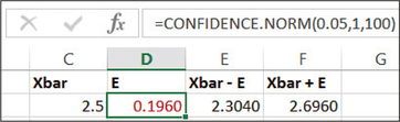
8.1.65
(a) (2.3040, 2.6960) (b) We are 95% confident that the population mean lies between 2.3040 and 2.6960. (c) 0.1960 (d) We can estimate the population mean to within 0.1960 with 95% confidence.
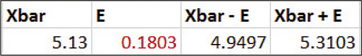
Question 8.66
66. Purchase Visits. In the Excel output, represents the population mean number of purchase visits made, per customer, over six months. The confidence level is 95%.
Question 8.67
67. Fourth-Graders' Feet. For the CrunchIt! Output, represents the population mean length of fourth-graders' feet, in cm.
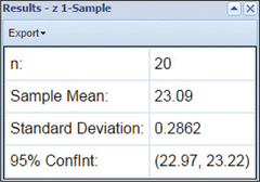
8.1.67
(a) (22.97, 23.22) (b) We are 95% confident that the population mean lies between 22.97 and 23.22. (c) 0.125 (d) We can estimate the population mean to within 0.125 with 95% confidence.
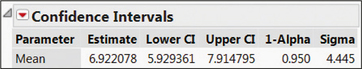
Question 8.68
68. Sugar Content in Breakfast Cereal. For the JMP output, represents the population mean amount of sugars, in grams, for all breakfast cereals.
Question 8.69
carbon
69. Carbon Emissions. The following table represents the carbon emissions (in millions of tons) from consumption of fossil fuels for a random sample of five nations.3 Assume .
| Nation | Emissions |
|---|---|
| Brazil | 361 |
| Germany | 844 |
| Mexico | 398 |
| Great Britain | 577 |
| Canada | 631 |
- Assess the normality of the data, using a normal probability plot. (Hint: See page 381.) Confirm that the conditions for constructing a interval are met.
- Assuming that carbon emissions are normally distributed, construct and interpret a 90% confidence interval for the population mean carbon emissions.
- Calculate and interpret the margin of error for the confidence interval in part (b).
- How large a sample size do we need to estimate to within 50 million tons with 90% confidence?
8.1.69
(a) The normal probability plot indicates an acceptable level of normality.
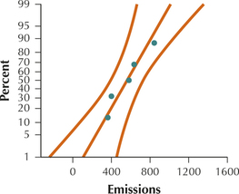
(b) (415.067, 709.333); TI-83/84: (415.08, 709.32). We are 90% confident that the population mean carbon emissions lies between 415.067 (415.08) million tons and 709.333 (709.32) million tons. (c) million tons. We can estimate the population mean emissions level of all nations to within 147.133 million tons with 90% confidence. (d) 44 nations
Question 8.70
deepwaterclean
70. Deepwater Horizon Cleanup Costs. The following table represents the amount of money distributed by BP a random sample of six Florida counties for cleanup of the Deepwater Horizon oil spill, in millions of dollars.4 Assume .
| County | Cleanup costs ($ millions) |
|---|---|
| Broward | 0.85 |
| Escambia | 0.70 |
| Franklin | 0.50 |
| Pinellas | 1.15 |
| Santa Rosa | 0.50 |
| Walton | 1.35 |
- Assess the normality of the data, using a normal probability plot. Confirm that the conditions for constructing a interval are met.
- Assuming that the cleanup costs are normally distributed, construct and interpret a 95% confidence interval for the population mean cleanup cost.
- Calculate and interpret the margin of error for the confidence interval in part (b).
- How large a sample size do we need to estimate to within $50,000 with 95% confidence?
Question 8.71
georgiarain
71. A Rainy Month in Georgia? The following table represents the total rainfall (in inches) for the month of February 2011 for a random sample of 10 locations in Georgia.5 Assume .
| Location | Rainfall (inches) |
Location | Rainfall (inches) |
|---|---|---|---|
| Athens | 4.72 | Atlanta | 4.25 |
| Augusta | 4.31 | Cartersville | 3.03 |
| Dekalb | 2.96 | Fulton | 4.36 |
| Gainesville | 4.06 | Lafayette | 3.75 |
| Marietta | 3.20 | Rome | 3.26 |
- Assess the normality of the data, using a normal probability plot.
- Assuming that the rainfall amounts are normally distributed, construct and interpret a 95% confidence interval for the population mean rainfall in inches.
- Calculate and interpret the margin of error for the confidence interval in part (b).
- How large a sample size do we need to estimate to within 0.1 inch with 95% confidence?
8.1.71
(a) The normal probability plot indicates an acceptable level of normality.
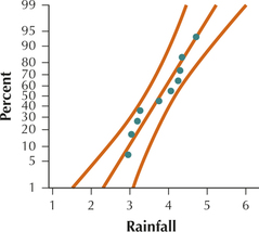
(b) (3.393, 4.187). We are 95% confident that the population mean rainfall in Georgia lies between 3.393 inches and 4.187 inches. (c) inch. We can estimate the population mean rainfall in Georgia to within 0.397 inch with 95% confidence. (d) 158 locations
Question 8.72
72. Short-term Memory. In a famous research paper in the psychology literature, George Miller found that the amount of information humans could process in short-term memory was 7 bits (pieces of information), plus or minus 2 bits.6 Let us assume that the title of Miller's paper (“The Magical Number Seven, Plus or Minus Two”) refers to a confidence interval. Assume that .
447
- What is the point estimate for the amount of information all humans can process in short-term memory?
- What is the margin of error? Interpret this number.
- The most common confidence level in the psychological literature is 95%. Which value for is associated with 95% confidence?
- How large a sample size did Miller use to find the confidence interval in the title, assuming that he used 95% confidence?
- Suppose he had wanted the title to read “The Magical Number Seven, Plus or Minus One”? How large a sample size would he have needed?
Question 8.73
commutedist
73. Commuting Distances. A university is trying to attract more commuting students from the local community. As part of the research into the modes of transportation students use to commute to the university, a survey was conducted asking how far commuting students commuted from home to school each day. A random sample of 30 students provided the distances (in miles) shown in the table below. Assume that the standard deviation is miles.
| 14 | 10 | 14 | 12 | 12 | 11 | 5 | 6 | 9 | 14 | 9 | 9 | 4 | 7 | 15 |
| 9 | 7 | 7 | 12 | 10 | 15 | 10 | 6 | 11 | 9 | 11 | 10 | 11 | 7 | 12 |
- Compute and interpret the margin of error for a confidence interval with 95% confidence.
- Construct and interpret a 95% confidence interval for the population mean commuting distance.
8.1.73
(a) miles. We can estimate μ, the mean commuting distance, to within 1.07 miles with 95% confidence. (b) (8.86, 11.00). We are 95% confident that the true mean commuting distance lies between 8.86 miles and 11.00 miles.
Question 8.74
74. Herbicide Concentration. Human exposure to herbicides is a potential hazard in America's grain-producing areas. One study found that, in a random sample of 112 homes in Iowa, the median concentration of the herbicide dicamba was 179.5 ng/g (nanograms per gram).7 Suppose that the sample mean was 180 ng/g, and assume that the population standard deviation is 20 ng/g.
- Compute and interpret the margin of error for a confidence interval with 95% confidence.
- Construct and interpret a 95% confidence interval for the population mean concentration of the herbicide dicamba in Iowa homes.
- How large a sample size is needed to estimate to within 3.7 ng/g with 95% confidence? Comment.
- How large a sample size is needed to estimate to within 3.7 ng/g with 99% confidence?
Question 8.75
75. Asthma and Quality of Life. A study examined the relationship between perceived neighborhood problems, quality of life, and mental health among adults with asthma.8 Among those reporting the most serious neighborhood problems, the 95% confidence interval for the population mean quality of life score was (2.7152, 9.1048).
- What is ?
- Find .
- Compute and interpret the margin of error.
- Suppose . Find the value for .
8.1.75
(a) (b) 5.91 (c) 3.1948. We can estimate the true mean quality of life score within 3.1948 with 95% confidence. (d) 9.78
Question 8.76
76. TV Viewing and Physical Activity. A study examined the relationship between television viewing and physical activity.9 The study found that, for each additional hour of television viewing, subjects walked between 12 and 276 fewer steps that day, as measured by a pedometer. This interval was reported with a 95% confidence level; suppose .
- What is ?
- Find .
- Compute and interpret the margin of error.
- Find the value for .
Question 8.77
77. Lead Contamination in Trout. The Washington State Department of Ecology reported that the mean lead contamination in trout in the Spokane River is 1 part per million (ppm), with a standard deviation of 0.5 ppm.10 Suppose a sample of trout has a mean lead contamination of . Assume that .
- Determine whether the requirements are met for constructing the interval for .
- Construct a 95% confidence interval for , the population mean lead contamination in all trout in the Spokane River.
- Interpret the confidence interval.
8.1.77
(a) and the population standard deviation is known. (b) (0.902, 1.098) (c) We are 95% confident that μ, the population mean lead contamination for all trout on the Spokane River, lies between 0.902 ppm and 1.098 ppm.
Question 8.78
 78. Refer to Exercise 77. What if the sample size is increased to some unspecified higher number. Describe what effect, if any, the increase has on the following:
- Width of the confidence interval
- Margin of error
- confidence level
Question 8.79
79. Refer to Exercise 77. What if the confidence level is decreased from 95% to some unspecified lower value. Explain whether and how this decrease would affect the following:
- Width of the confidence interval
- Margin of error
8.1.79
(a) Since is a population characteristic, it stay constant and is unaffected by a decrease in confidence level. (b) The quantity is unaffected by a decrease in confidence level. (c) A decrease in the confidence level will result in a decrease in . The width of the confidence interval . Thus a decrease in will result in a decrease in the width of the confidence interval. (d) The quantity depends only on the sample taken, so it will remain unaffected by a decrease in the confidence level. (e) A decrease in the confidence level will result in a decrease in . Since the margin of error is a decrease in will result in a decrease in the margin of error.
BRINGING IT ALL TOGETHER
Wii Game Sales. The following table represents the number of units sold in the United States for the week ending March 26, 2011, for a random sample of eight Wii games.11 Assume . Use this information for Exercises 80–85.
| Game | Units (1000s) |
Game | Units (1000s) |
|---|---|---|---|
| Wii Sports Resort | 65 | Zumba Fitness | 56 |
| Super Mario All Stars |
40 | Wii Fit Plus | 36 |
| Just Dance 2 | 74 | Michael Jackson | 42 |
| New Super Mario Brothers |
16 | Lego Star Wars | 110 |
448
Question 8.80
wiisales
80. Assess the normality of the data, using a normal probability plot.
Question 8.81
wiisales
81. Determine whether a interval may be used to estimate the population mean number of units sold.
8.1.81
The distribution is approximately normal and is known.
Question 8.82
wiisales
82. Find for 99% confidence.
Question 8.83
wiisales
83. Assuming that the game sales are normally distributed, construct and interpret a 99% confidence interval for the population mean number of units sold.
8.1.83
(27.6, 82.2). We are 99% confident that μ, the population mean Wii game sales, lies between 27.6 thousand units and 82.2 thousand units.
Question 8.84
wiisales
84. Calculate and interpret the margin of error for the confidence interval in Exercise 83.
Question 8.85
wiisales
85. How large a sample size do we need to estimate to within 5000 units with 99% confidence?
8.1.85
239 games
WORKING WITH LARGE DATA SETS
Small Businesses. Use this information for Exercises 86–90. The U.S. Small Business Administration publishes data on the number of small businesses in each of 327 metropolitan areas. This data is in the data file Small Businesses.
.
Question 8.86
smallbusinesses
86. Find the sample mean number of small firms per metropolitan area.
Question 8.87
smallbusinesses
87. Generate a histogram of the number of small firms per metropolitan area.
8.1.87
See the histogram in the answer for exercise 90.
Question 8.88
smallbusinesses
88. Generate a normal probability plot of the number of small firms in each metropolitan area. What is your conclusion regarding the normality of the distribution of the number of firms?
Question 8.89
smallbusinesses
89. Construct and interpret a 95% confidence interval for the population number of small firms per metropolitan area. Assume that the standard deviation is 25,000 firms.
8.1.89
(3189, 9209). We are 95% confident that the average number of small firms per metropolitan area lies between 3189 and 9209.
Question 8.90
smallbusinesses
90. On the histogram, indicate the location of the confidence interval.
![]() Use the Confidence Interval applet for Exercise 91.
Use the Confidence Interval applet for Exercise 91.
Question 8.91
91. Set the confidence level to 90%. Click “Sample 50” to produce 50 simple random samples (SRSs) and display the resulting 90% confidence intervals for .
- What is the percent hit, that is, the proportion of the confidence intervals that actually contain the true value of ?
- Keep clicking “Sample 50” until 1000 confidence intervals are generated. What is the percent hit?
- It is not likely (though it is possible) that the percent hit in (b) exactly equals 90%. Explain why the percent hit is not equal to 90% when we asked for a confidence level of 90%.
8.1.91
Answers will vary.
![]() Use the Normal Density Curve applet for Exercise 92.
Use the Normal Density Curve applet for Exercise 92.
Question 8.92
92. Use the applet to find critical values for unusual confidence levels. Select 2-Tail, and click and drag the flags so that the central area, not the tail area, is highlighted. Verify that the critical value for 95% confidence is 1.96.
Use the applet to find critical values for the following confidence levels:
- 80%
- 85%
- 98%
 Chapter 8 Case Study: Motor Vehicle Fuel Efficiency.
Open the Chapter 8 Case Study data set Fuel Efficiency. Here, we will examine confidence intervals for the population mean combined MPG (city and highway) generated by two different samples. We will then see whether these confidence intervals succeeded in capturing the population mean combined MPG. The population standard deviation is . Use technology to do the following:  fueleffciency
Question 8.93
93. Obtain a random sample of size 100 from the data set.
8.1.93
Answers will vary.
Question 8.94
94. Construct and interpret a 90% Z interval for the population mean combined MPG.
Question 8.95
95. Did your interval in Exercise 94 capture the population mean? Check by finding the mean combined MPG of all the vehicles in the entire data set.
8.1.95
Answers will vary.
Question 8.96
96. Generate a second sample of size 100 from the data set. Construct a second 90% interval for the population mean combined MPG. Did this confidence interval capture the population mean?
Question 8.97
97. If we keep on obtaining new samples all day long, about what proportion of the 90% confidence intervals will capture the population mean?
8.1.97
0.90