Appendix A: Answers to Your Turn Exercises
Chapter 13
A-1
YOUR TURN #1
Section 1.2, page 9
- The variable type takes the following values: adventure, platform, sports, shooter, action, role-playing, and racing.
- The observation for Spiderman 2 for PS4 is as follows:
Game Platform Studio Type Sales
for WeekSales
TotalWeeks
on ListSpiderman 2 t
for PS4PS4 Activision Action 6510 49,292 3
YOUR TURN #2
Section 1.2, page 10
- Since Sirius XM is a stock, it is an element.
- Another name for the variable Exchange would be Market.
YOUR TURN #3
Section 1.2, page 10
- Because the number of medals won is finite, the variable number of medals won is discrete.
- Because the time to run a 100-meter dash can take on an infinite number of values, the variable racing time in the 100-meter dash is continuous.
YOUR TURN #4
Section 1.2, page 11
- Exchange represents nominal data, because the data cannot be ordered in a natural or obvious way. Also, no arithmetic can be performed on exchange.
- Last price represents ratio data. Here division makes sense. A last price of $20 is twice a last price of $10.
YOUR TURN #5
Section 1.2, page 13
- Since Florida has more than 3 counties, this represents a sample.
- Since we are talking about all of the counties in Florida, this represents a population.
YOUR TURN #6
Section 1.2, page 13
- Since this represents a sample, the most expensive hotel in the 3 counties represents a statistic.
- Since this represents a population, the most expensive hotel in Florida represents a parameter.
YOUR TURN #7
Section 1.2, page 15
- The average grade on the first quiz is a descriptive statistic, since the average grade is only for your class. However, no inference is made regarding a larger population.
- Jessica won 2 out of 10 games of ping pong to her friend Lu Li. Therefore she won of her ping pong games to Lu Li. This represents a statistic. She then used this statistic to perform statistical inference to conclude that she will only win 20% of her games of ping pong to Lu Li.
YOUR TURN #8
Section 1.3, page 23
- Systematic sample: Bill Gates, Charles Koch, Jim Walton, Michael Bloomberg, Larry Page, Jacqueline Mars, George Soros
- Systematic sample: Larry Ellison, Alice Walton, Larry Page, Carl Icahn
YOUR TURN #9
Section 1.3, page 25
- Since you used a random sample from your school, this is not convenience sampling.
- Since you obtain data from your 5 closest friends at school, this is convenience sampling. You are choosing a sample that is convenient for you.
YOUR TURN #10
Section 1.3, page 26
- Convenience sampling: you are choosing a sample convenient for you.
- Systematic Sampling: where every kth student is taken, with .
- Cluster sampling: (a) the population was divided into clusters (classes), (b) a random sample of one cluster (class) is taken, and (c) every student in that cluster (class) is selected.
- Stratified sampling: (a) the population was divided into subgroups (nursing majors and all others), and (b) a random sample from each of the groups was drawn.
- Random sampling: the two names were selected randomly.
Chapter 2
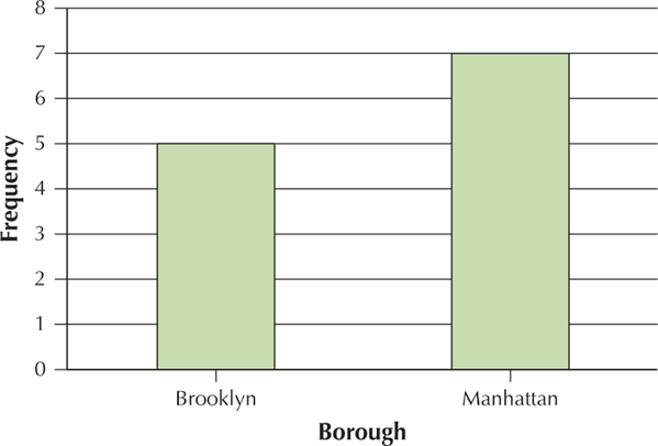
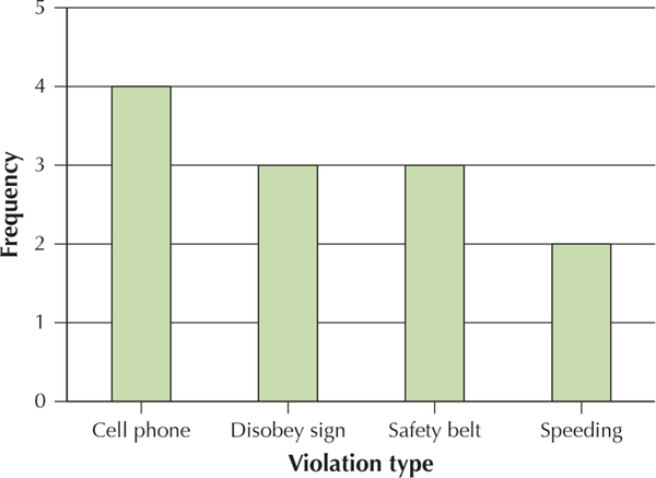
YOUR TURN #1
Section 2.1, page 41
Borough Frequency Brooklyn 5 Manhattan 7 Violation type Frequency Cell phone 4 Safety belt 3 Speeding 2 Disobey sign 3
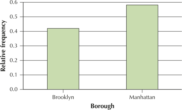
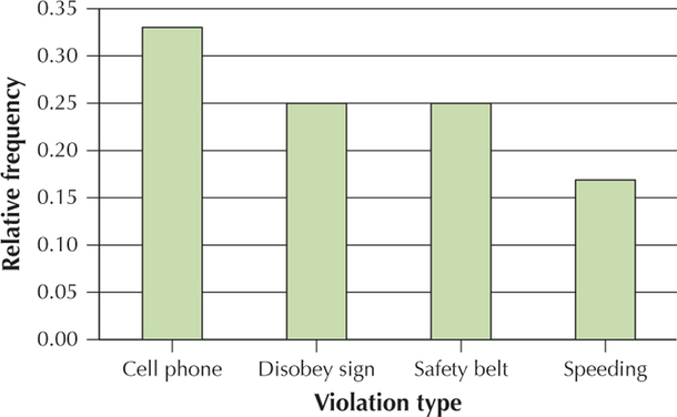
YOUR TURN #2
Section 2.1, page 42
Borough Relative frequency Brooklyn Manhattan Violation type Relative frequency Cell phone Safety belt Speeding Disobey sign
A-2
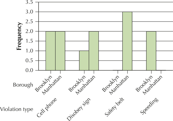
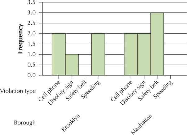
YOUR TURN #3
Section 2.1, page 43
YOUR TURN #4
Section 2.1, page 47
| Violation type | |||||
|---|---|---|---|---|---|
| Borough | Cell phone |
Disobey sign |
Safety belt |
Speeding | Total |
| Brooklyn | 2 | 1 | 0 | 2 | 5 |
| Manhattan | 2 | 2 | 3 | 0 | 7 |
| Total | 4 | 3 | 3 | 2 | 12 |
YOUR TURN #5
Section 2.1, page 48
- (a)
SAT Writing score Frequency 200–390 347,920 400–590 1,015,121 600–800 297,006 Total 1,660,047 - (b)
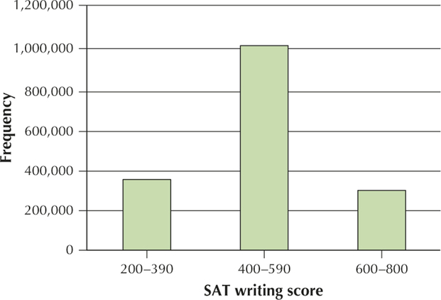
YOUR TURN #6
Section 2.1, page 49
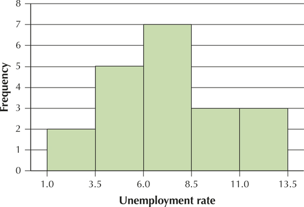
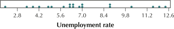
YOUR TURN #7
Section 2.2, pages 64–65
Class boundaries: 1 to < 3.5, 3.5 to < 6, 6 to < 8.5, 8.5 to <11, 11 to < 13.5
| Class: | Frequency | Relative frequency |
|---|---|---|
| 2 | ||
| 5 | ||
| 7 | ||
| 3 | ||
| 3 | ||
| Table | 3 |
A-3
YOUR TURN #8
Section 2.2, page 66
YOUR TURN #9
Section 2.2, page 68
YOUR TURN #10
Section 2.2, page 69
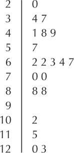
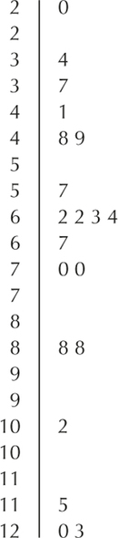
YOUR TURN #11
Section 2.2, page 70
YOUR TURN #12
Section 2.2, page 72
- No. The class boundaries are from 6 to 8.5.
- 3
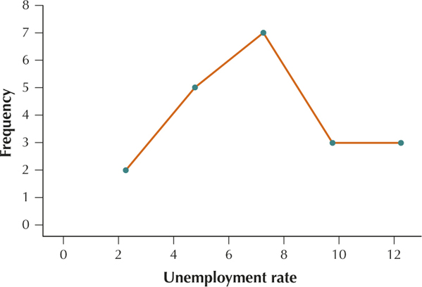
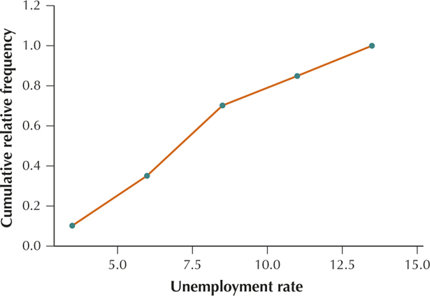
YOUR TURN #13
Section 2.3, page 88
| Unemployment rate |
Frequency | Relative frequency |
Cumulative frequency |
Cumulative relative frequency |
|---|---|---|---|---|
| 2 | 2 | 0.10 | ||
| 5 | ||||
| 7 | ||||
| 3 | ||||
| 3 | ||||
| Total | 20 |
YOUR TURN #14
Section 2.3, page 89
Chapter 3
YOUR TURN #1
Section 3.1, page 109
Mean number of tropical storms =
The population mean number of tropical storms is 15.125 storms.
YOUR TURN #2
Section 3.1, page 110
- (a) The sample mean would be lower than $337.50 without the Sony Xperia Z2 since the price of this phone is $600, which is higher than the prices of the other phones.
- . Yes, the sample mean of $250 is lower than $337.50.
A-4
YOUR TURN #3
Section 3.1, page 115
The sample consists of the number of tropical storms in the years 2006, 2008, 2010, and 2012: 10, 16, 19, 19
The mean is .
The data set is already in ascending order.
Because is even, the median is the mean of the two data values that lie on either side of the position. That is, the median is the mean of the 2nd and 3rd data values, 16 and 19. Splitting the difference between these two, we get median number of tropical storms storms.
Since 19 storms appears two times and no other number appears more than once, the mode is 19.
YOUR TURN #4
Section 3.2, page 128
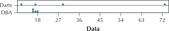
- Darts has the larger range.
As we expected, the range for Darts is indeed larger than the range for DJIA.
YOUR TURN #5
Section 3.2, page 131
7.8 7.4529 1.9 10.0489 14.9 96.6289 1.5 12.7449 2.7 5.6169 1.6 12.0409
From the table,
YOUR TURN #6
Section 3.2, page 132
From Your Turn #5 on p. 131, the population variance is . Therefore the population standard deviation is
YOUR TURN #7
Section 3.2, page 134
From Table 14 on p. 130, the CDC provided $1.9 million to Maine, $1.5 to New Hampshire, and $1.6 million to Vermont to fight HIV/AIDS. Therefore our sample data is: $1.9 million, $1.5 million, $1.6 million
- Smaller. The sample contains the 3 smallest numbers in the population.
First we need to find the sample mean.
1.5 0.0289 1.9 0.0529 1.6 0.0049 From the table, . Therefore the sample variance is billion of dollars squared.
- From Problem 2 the sample variance is billion of dollars squared. Therefore the sample standard deviation is .
- For this sample of CDC funding to fight HIV/AIDS in the northeastern United States, the typical difference between a state's funding and the mean funding is $0.2082 billion.
YOUR TURN #8
Section 3.2, page 137
- mph and m mph Therefore the percentage of vehicle speeds that lie between 65 mph and 75 mph is the percentage of vehicle speeds that lie within 1 standard deviation of the mean. Thus, from the Empirical Rule, approximately 68% of vehicle speeds lie between 65 mph and 75 mph.
- From Problem 1, 65 mph lies 1 standard deviation below the mean. Therefore the Empirical Rule tells us that of all vehicle speeds are at most 65 mph.
YOUR TURN #9
Section 3.2, page 139
Since and . Therefore Chebyshev's Rule tells us that at least of the systolic blood pressure readings will lie between 110 and 150.
YOUR TURN #10
Section 3.3, page 149
The data values are 90, 70, and 85. The weights are 50, 20, and 30. The course weighted mean is then calculated as follows:
YOUR TURN #11
Section 3.4, page 156
The amount Austin spent on video games is .
The amount Brian spent on music downloads is .
The amount Courtney spent on gifts for her friends is .
A-5
YOUR TURN #12
Section 3.4, page 157
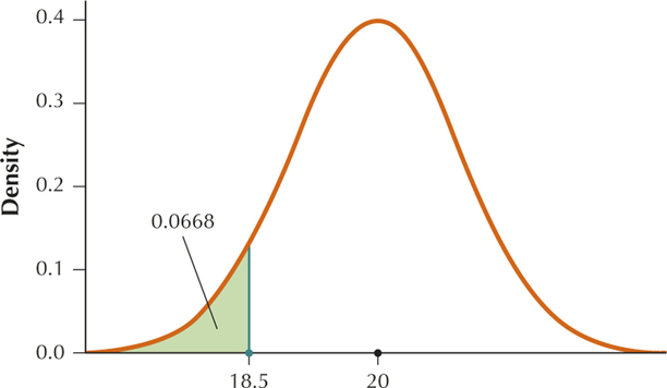
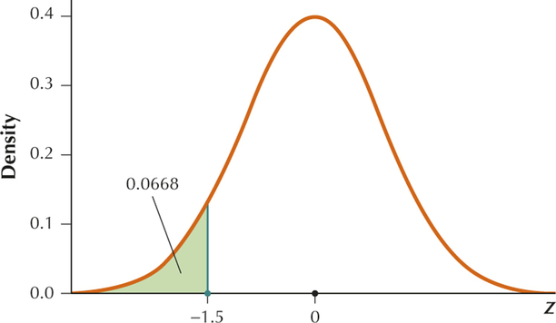
David's -score was −1.5. Therefore he spent
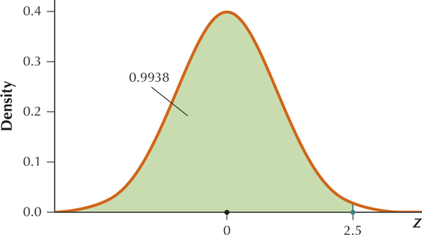
Emily's -score was 2.5. Therefore she spent
Frances's -score was 0. Therefore she spent
YOUR TURN #13
Section 3.4, page 158
Gisele used a tablet. Note here that we have population values, with and . The amount Gisele spent on an online holiday shopping order is .
Hong used a cell phone. Note here that we have population values, with and . The amount Hong spent on an online holiday shopping order is .
Since the -score for Hong is larger than the -score for Gisele, Hong spent more relative to his group.
YOUR TURN #14
Section 3.4, page 159
- Austin's -score is 1, which lies in the range, −2 , -score < 2. Therefore the amount Austin spent on video games is not considered unusual.
- Brian's -score is −2, which lies in the range, −3 , -score ≤ −2. Therefore the amount Brian spent on music downloads may be considered moderately unusual.
- Courtney's -score is 4, which is ≥3. Therefore the amount Courtney spent on gifts for her friends may be considered an outlier.
YOUR TURN #15
Section 3.4, page 161
| Position | 1 | 2 | 3 | 4 | 5 | 6 | 7 | 8 | 9 |
|---|---|---|---|---|---|---|---|---|---|
| Rating | 1.9 | 2.5 | 3.6 | 4.2 | 5.4 | 5.7 | 7.1 | 8.7 | 9.3 |
Since there are 9 numbers, . Since we want the number corresponding to the 20th percentile, . Thus .
Here, is not an integer, so round up to 2. The 20th percentile is the number in position 2, which is 2.5. Thus, the 20th percentile is 2.5.
YOUR TURN #16
| Position | 1 | 2 | 3 | 4 | 5 | 6 | 7 | 8 | 9 |
|---|---|---|---|---|---|---|---|---|---|
| Rating | 1.9 | 2.5 | 3.6 | 4.2 | 5.4 | 5.7 | 7.1 | 8.7 | 9.3 |
Here, . Eight of the movies have a ranking of 9.0 or below, so the percentile rank of a movie with a rating of 9.0 or below is
Percentile rank of data value
Thus a rating of 9 represents the 89th percentile of movie ratings.
YOUR TURN #17
Section 3.4, page 164
| Position | 1 | 2 | 3 | 4 | 5 | 6 | 7 | 8 | 9 |
|---|---|---|---|---|---|---|---|---|---|
| Rating | 1.9 | 2.5 | 3.6 | 4.2 | 5.4 | 5.7 | 7.1 | 8.7 | 9.3 |
Here, . To find Q1, plug into , where . We get . Here, is not an integer so round up to 3. The 25th percentile is the number in position 3, which is 3.6. Thus Q1, the 25th percentile, is 3.6.
To find Q2 = the median, plug into , where . We get . Here, is not an integer so round up to 5. The 50th percentile is the number in position 5, which is 5.4. Thus Q2 = the median, the 50th percentile, is 5.4.
To find Q3, plug into , where . We get . Here, is not an integer so round up to 7. The 75th percentile is the number in position 7, which is 7.1. Thus Q3, the 75th percentile, is 7.1.
YOUR TURN #18
Section 3.4, page 166
From Your Turn #17 on p. 164, and . Thus .
YOUR TURN #19
Section 3.5, page 172
| Position | 1 | 2 | 3 | 4 | 5 | 6 | 7 | 8 | 9 |
|---|---|---|---|---|---|---|---|---|---|
| Rating | 1.9 | 2.5 | 3.6 | 4.2 | 5.4 | 5.7 | 7.1 | 8.7 | 9.3 |
From Your Turn #17, p. 164,, the , and . From the table, the minimum is 1.9 and the maximum is 9.3. Thus, the five-number summary is:
- Minimum = 1.9
- First quartile, Q1 = 3.6
- Median = Q2 = 5.4
- Third quartile, Q3 = 7.1
- Maximum = 9.3
YOUR TURN #20
Section 3.5, page 175
From Your Turn #19 on p. 172, the five-number summary is:
- Minimum = 1.9
- First quartile, Q1 = 3.6
- Median = Q2 = 5.4
- Third quartile, Q3 = 7.1
- Maximum = 9.3
The .
The lower fence .
The upper fence .
A-6
YOUR TURN #21
Section 3.5, page 178
From Your Turn # 20 on p. 175:
The lower fence .
The upper fence .
Thus, for this data set, a data value would be an outlier if it is −1.65 or less or 12.35 or more. Since none of the data values are −1.65 or less or 12.35 or more there are no outliers in this data set.
Chapter 4
YOUR TURN #1
Section 4.1, page 189
Because the response variable depends on the predictor variable, and because the grade on an exam depends in part on the number of hours spent studying for the exam, the number of hours spent studying for the exam is the predictor () variable and the grade on the exam is the response () variable.
YOUR TURN #2
Section 4.1, page 190
- Because the response variable depends on the predictor variable, and because the weight of a person depends in part on the height of the person, height is the predictor () variable and weight is the response () variable.
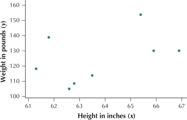
YOUR TURN #3
Section 4.1, page 192
Height and weight have a positive linear relationship.
YOUR TURN #4
Section 4.1, page 194
Step 1
Step 2
63.5 113.8 −0.275 0.075625 −11 121 3.025 65.9 130.1 2.125 4.515625 5.3 28.09 11.2625 62.8 108.5 -0.975 0.950625 -16.3 265.69 15.8925 61.8 138.9 -1.975 3.900625 14.1 198.81 -27.8475 61.3 118.2 -2.475 6.125625 -6.6 43.56 16.335 66.9 130.1 3.125 9.765625 5.3 28.09 16.5625 62.6 104.9 -1.175 1.380625 -19.9 396.01 23.3825 65.4 153.9 1.625 2.640625 29.1 846.81 47.2875 Step 3
Step 4
YOUR TURN #5
Section 4.1, page 198
From Your Turn #4, p. 194, . Since is positive, we would therefore say that height and weight are positively correlated. As height increases, weight also tends to increase.
YOUR TURN #6
Section 4.2, page 211
- (a) From Your Turn #4, page 194:
- Step 1 Calculate the respective sample means and . We have already done this in Your Turn #4 (page 194): inches and pounds.
- Step 2 Calculate the respective sample standard deviations and . We have already done this in Your Turn #4 (page 194): .
- Step 3 Find the correlation coefficient . We have already done this in Your Turn #4 (page 194): .
Step 4 Combine the statistics from Steps 2 and 3 to calculate :
- (b)
- (c) Because and represent weight and height, respectively, this regression equation is read as follows: “The estimated weight of a woman is 3.6076 times her height minus 105.2723 pounds.”
YOUR TURN #7
Section 4.2, page 211
- (a) For a woman with height 0 inches, her estimated weight is −105.2723 pounds.
- (b) For each increase of 1 inch to a woman's height, her estimated weight increases by 3.6076 pounds.
YOUR TURN #8
Section 4.2, page 213
In Your Turn #7 (page 211), we calculated the regression equation to be . Therefore, for a woman who is inches tall, her estimated weight is pounds.
YOUR TURN #9
Section 4.2, page 215
In Your Turn #8 (page 213), the estimated weight for a woman who is inches tall is pounds. From Table 2 on page 190, the actual weight of the woman who is inches tall is pounds. Therefore the prediction error is pounds. Since the prediction error is negative, her actual weight lies below the regression line.
A-7
YOUR TURN #10
Section 4.2, page 216
From Table 2, the smallest value of is 61.3 inches and the largest is 66.9 inches, so estimates for any value of between 61.3 inches and 66.9 inches, inclusive, would not represent extrapolation.
- (a) For inches, pounds. Because inches lies between 61.3 inches and 66.9 inches, inclusive, this estimate does not represent extrapolation.
- (b) For inches, pounds. Because inches does not lie between 61.3 inches and 66.9 inches, this estimate represents extrapolation.
Chapter 5
YOUR TURN #1
Section 5.1, page 243
- (a) The chance of a recession near zero means that the probability of a recession is near zero. Therefore it is very unlikely that a recession will occur.
- (b) The chance of satisfaction with the purchase of a new car is 100% means the probability that you will be satisfied with the purchase of a new car is 1. Therefore it is certain that you will be satisfied with the purchase of a new car.
YOUR TURN #2
Section 5.1, page 245
- (a) A total of 52 outcomes is included in the sample space, so Let be the event a heart is drawn. Then consists of the 13 hearts
 so . Therefore the probability of drawing a heart is .
 - (b) A total of 52 outcomes is included in the sample space, so . Let be the event a black card is drawn. Then consists of the 26 black cards
 so . Therefore the probability of drawing a black card is .
YOUR TURN #3
Section 5.1, page 245
- (a) Since only a roll of 6 wins, the other 5 possible rolls {1, 2, 3, 4, 5} don't win. Therefore the probability of not winning is .
- (b) There are 6 possible rolls. Only one of them is a 5. Therefore the probability of rolling a 5 is .
YOUR TURN #4
Section 5.1, page 246
- (a)
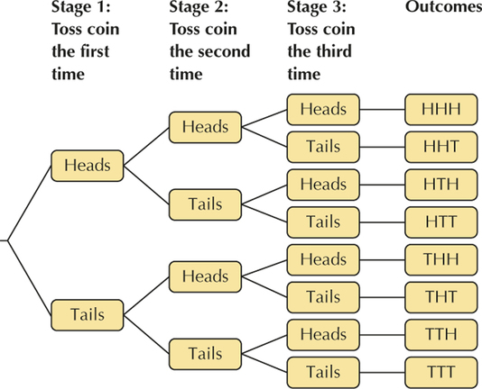
- (b) {HHH, HHT, HTH, HTT, THH, THT, TTH, TTT}
YOUR TURN #5
Section 5.1, page 247
- (a) Let be the event toss two heads. Then , so . Therefore .
- (b) Let be the event toss two tails. Then , so . Therefore .
YOUR TURN #6
Section 5.1, page 247
- (a) Let denote the event roll a sum of 7. Then consists of the outcomes {(1,6),(2,5),(3,4),(4,3),(5,2),(6,1)}, so . Therefore .
- (b) Let denote the event roll a sum of 12. Then F consists of the outcome {(6, 6)}, so . Therefore .
- (c) Let denote the event roll a sum of 2. Then consists of the outcome {(1,1)}, so . Therefore .
YOUR TURN #7
Section 5.1, page 250
- (a) Define : Patient did not complete treatment.
- (b) Relative frequency of .
- (c) .
YOUR TURN #8
Section 5.2, page 260
From Example 7 on page 247, .
- (a) consists of the outcomes {(2, 6), (3, 5), (4, 4), (5, 3), (6, 2)}, so . Therefore .
- (b) consists of all of the outcomes in the sample space that are not in . Therefore consists of the outcomes {(1,1), (1, 2), (1, 3), (1, 4), (1, 5), (1, 6), (2, 1), (2, 2), (2, 3), (2, 4), (2, 5), (3, 1), (3, 2), (3, 3), (3, 4), (3, 6), (4, 1), (4, 2), (4, 3), (4, 5), (4, 6), (5, 1), (5, 2), (5, 4), (5, 5), (5, 6), (6, 1), (6, 3), (6, 4), (6, 5), (6, 6)}, so . Therefore .
YOUR TURN #9
Section 5.2, page 262
- (a) The set ( and ) is the set of outcomes that are common to both and . The green cell belongs to both the Male column and the Person did not survive row. The green cell represents (M and Nd, which includes the 1364 males who did not survive.
Female Male Total Did not survive 126 1364 1490 Survived 344 367 711 Total 470 1731 2201 - (b) The set ( or ) is the set of outcomes that are in or or both. The green cells are the people that were either male or did not survive or both. Therefore ( or ) is represented by the green cells.
Female Male Total Did not survive 126 1364 1490 Survived 344 367 711 Total 470 1731 2201
A-8
YOUR TURN #10
Section 5.2, page 263
- (a) Here we seek . There were 1731 males out of a total of 2201 passengers aboard the Titanic. Therefore .
- (b) We are looking for . Of the 2201 passengers onboard, 1490 of them did not survive. Therefore .
- (c) Those who were both male and did not survive represent ( and ). From Your Turn #9, p. 262, there are 1364 out of the 2201 passengers who were male and did not survive. Therefore .
- (d) Here we seek . From the Addition Rule, .
YOUR TURN #11
Section 5.2, page 265
Here we seek (On Campus or Off Campus). Of the 19,375 students at the university, 2608 live on campus and 9911 live off campus. Thus and . Since no one is living both on campus and off campus at the same time, the events On Campus and Off Campus are mutually exclusive. From the Addition Rule for Mutually Exclusive Events,
YOUR TURN #12
Section 5.3, page 274
- (a) The event did not respond to the marketing campaign is the complement of the event responded to the marketing campaign. Therefore denotes the event did not respond to the marketing campaign. . We could have also used the formula for the probability of a complement. This gives us .
- (b) The event did not have a credit card on file is the complement of the event has a credit card on file. Therefore denotes the event does not have a credit card on file. Then .
YOUR TURN #13
Section 5.3, page 275
| Female | Male | Total | |
|---|---|---|---|
| Did not survive | 126 | 1364 | 1490 |
| Survived | 344 | 367 | 711 |
| Total | 470 | 1731 | 2201 |
Define the following events:
- : Person is male.
- : Person did not survive.
Then and . Since , and are not independent.
YOUR TURN #14
Section 5.3, page 277
Define the following events:
- : Roll a 6 on the first toss.
- : Roll a 6 on the second toss.
Then . Since the second toss of the die is not affected by the first toss of the die, and are independent. Therefore . Using the Multiplication Rule we have .
YOUR TURN #15
Section 5.3, page 277
. Using the Multiplication Rule for Independent Events, we get .
YOUR TURN #16
Section 5.3, p. 278
Define the following events:
- : Observe a heart on the first draw.
- : Observe a heart on the second draw.
Since we are sampling with replacement, and are independent. Then . Using the Multiplication Rule for Independent Events we get .
YOUR TURN #17
Section 5.3, page 279
Define the following events:
- : Observe a heart on the first draw.
- : Observe a heart on the second draw.
Since we are sampling without replacement, and are dependent. Then . After drawing a heart from the deck there are 51 cards left and 12 hearts left. Thus . Using the Multiplication Rule we get .
YOUR TURN #18
Section 5.3, page 281
YOUR TURN #19
Section 5.3, page 281
(At least 1 of the 4 Americans smokes)
YOUR TURN #20
Section 5.3, page 283
Define the following event:
: Used hospital-based insurance
Then using Bayes' Rule we get
A-9
YOUR TURN #21
Section 5.4, page 293
Once again no one can finish in more than one place. Therefore there is no repetition. Thus there are 6 · 5 · 4 · 3 = 360 possible sets of trophy winners.
YOUR TURN #22
Section 5.4, page 294
10 · 9 · 8 · 7 · 6 · 5 · 4 · 3 · 2 · 1 = 3,628,800
YOUR TURN #23
Section 5.4, page 294
- (a) 9! = 9 · 8 · 7 · 6 · 5 · 4 · 3 · 2 · 1 = 362,880
- (b) 10! = 10 · 9 · 8 · 7 · 6 · 5 · 4 · 3 · 2 · 1 = 3,628,800, as in Your Turn #22.
YOUR TURN #24
Section 5.4, page 295
10 · 9 · 8 · 7 · 6 = 30,240
YOUR TURN #25
Section 5.4, page 296
- (a)
- (b)
- (c)
YOUR TURN #26
Section 5.4, page 297
YOUR TURN #27
Section 5.4, page 298
- (a)
- (b)
- (c)
Chapter 6
YOUR TURN #1
Section 6.1, page 312
- (a) Your best friend's height is something that is measured, not counted. Therefore your best friend's height is a continuous variable. Possible values for your best friend's height in feet are .
- (b) The number of cats you have is something you count. Therefore the number of cats you have is a discrete variable. Possible values are {0,1,2,3,…}.
YOUR TURN #2
Section 6.1, page 314
All of the probabilities are between 0 and 1. However, the sum of the probabilities is , which is not equal to 1. Therefore this is not a valid discrete probability distribution.
YOUR TURN #3
Section 6.1, page 315
YOUR TURN #4
Section 6.1, page 315
- (a)
- (b) The outcomes and mutually exclusive. Therefore, .
- (c) The phrase at most means “that many or fewer.” Thus, .
- (d) The phrase at least means “that many or more.” Thus, .
YOUR TURN #5
Section 6.1, page 317
| = Number of heads | ||
|---|---|---|
| 0 | 0 · 0.25 = 0 | |
| 1 | 1 · 0.50 = 0.50 | |
| 2 | 2 · 0.25 = 0.50 | |
| Total |
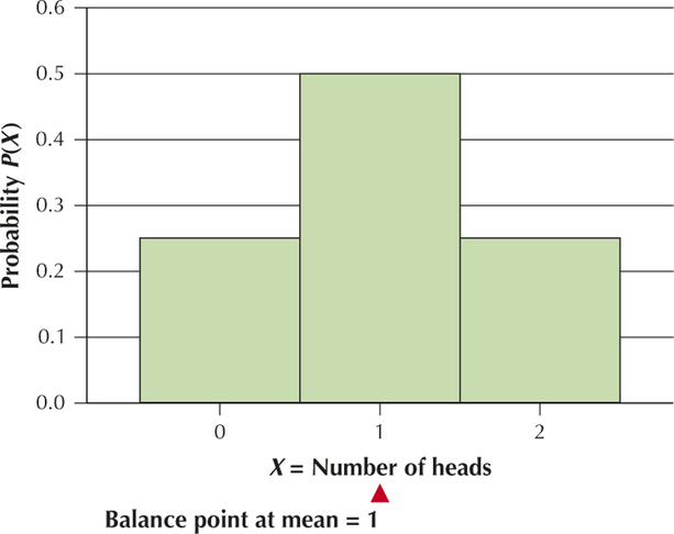
Therefore the mean number of heads is 1.
YOUR TURN #6
Section 6.1, page 318
YOUR TURN #7
Section 6.1, page 318
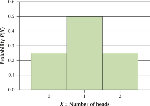
The largest probability in the table is and the largest bar in the graph in Your Turn #6 is for . Therefore the most likely number of heads is .
A-10
YOUR TURN #8
Section 6.2, page 331
- (a)
- (b)
- (c)
YOUR TURN #9
Section 6.2, page 334
(a)
From the TI-84 Plus: 0.623046875
(b)
From the TI-84 Plus: 0.623046875
(c) From the binomial table:
From the TI-84 Plus: 0.623046875
(d) From the binomial table:
From the TI-84 Plus: 0.3759765625
YOUR TURN #10
Section 6.2, page 335
- (a)
- (b)
- (c) We use the -score method. The -score for is is neither an outlier nor unusual.
YOUR TURN #11
Section 6.3, page 344
(a) Here, , so the probability that is
(b) Here, , so the probability that is
YOUR TURN #12
Section 6.3, page 345
- (a) Mean = μ = 10, Variance = = 10, Standard deviation = .
(b) A data value farther than 2 standard deviations from the mean is considered moderately unusual. The number of customers to a boutique shop that lie 2 standard deviations above and below the mean are calculated as follows:
Thus if there were 3 or less customers to the boutique shop this would be considered moderately unusual. Similarly, if there were 17 or more customers to the boutique shop this would also be considered moderately unusual.
YOUR TURN #13
Section 6.4, page 351
YOUR TURN #14
Section 6.4, page 356
YOUR TURN #15
Section 6.4, page 357
YOUR TURN #16
Section 6.4, page 360
A-11
YOUR TURN #17
Section 6.4, page 361
YOUR TURN #18
Section 6.4, page 362
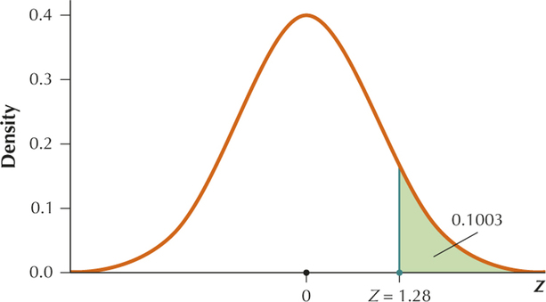
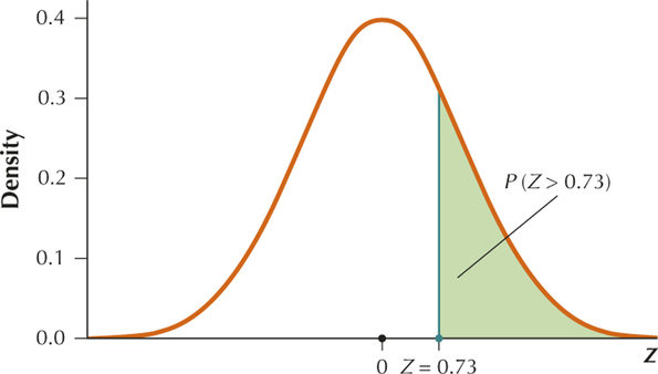
YOUR TURN #19
Section 6.5, page 370
We want . Thus we want to find the area shaded in the graph below.
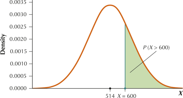
Standardizing we get
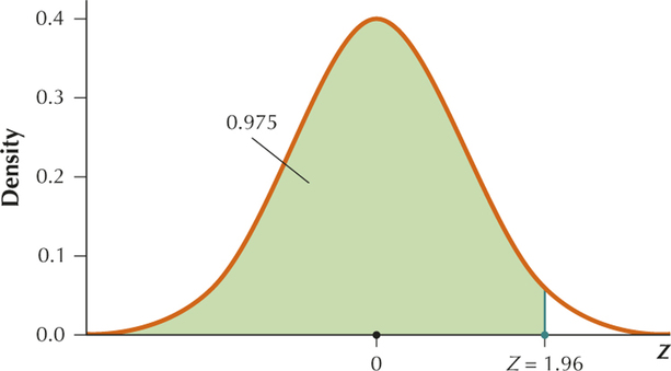
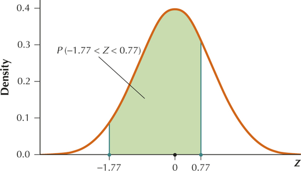
YOUR TURN #20
Section 6.5, page 372
We want to find .
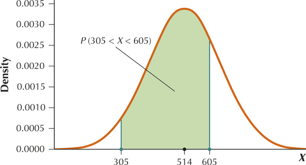
Standardizing we get
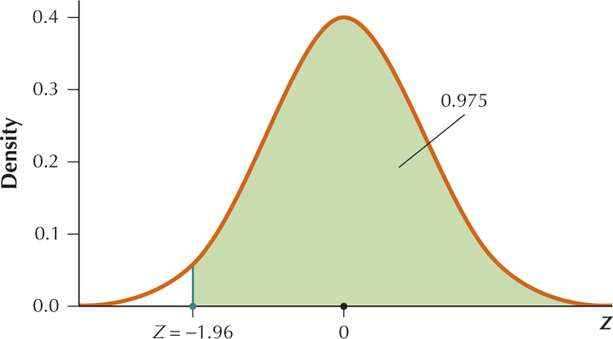
YOUR TURN #21
Section 6.5, page 373
From the table . Then .
A-12
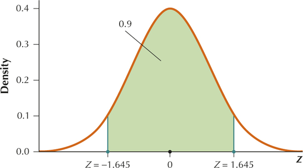
YOUR TURN #22
Section 6.5, page 374
From the table, . Then .
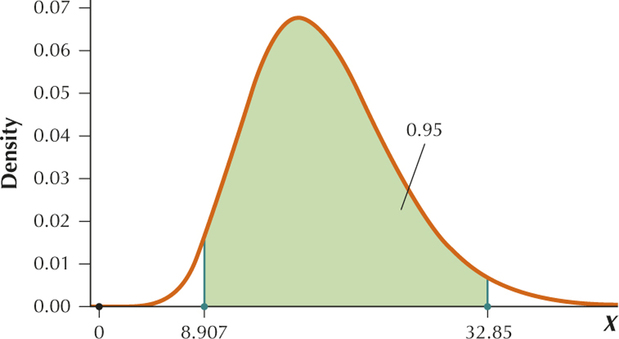
YOUR TURN #23
Section 6.6, page 389
Chapter 7
YOUR TURN #1
Section 7.1, page 399
We have .
YOUR TURN #2
Section 7.1, page 403
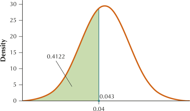
We want to find .
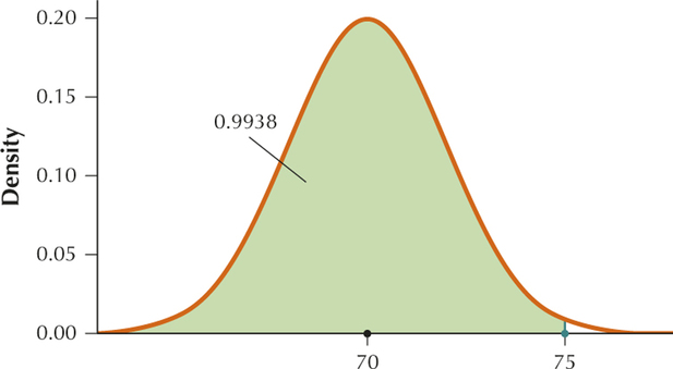
From Example 5, page likes and page likes.
Therefore
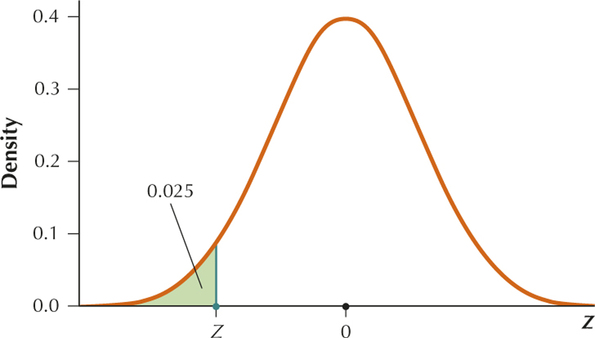
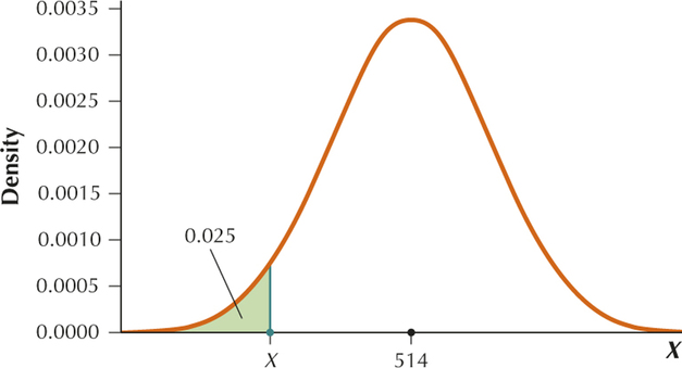
YOUR TURN #3
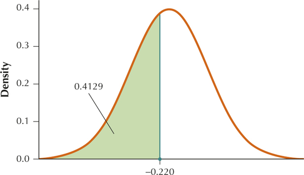
Section 7.1, page 405
From Example 5, page likes and page likes. We want the 2.5th percentile, so we look for 0.0250 on the inside of the table. Working backward from 0.0250 we find that . Thus .
YOUR TURN #4
Section 7.1, page 406
From Example 7, and . We want to find .
Standardizing, we get
Therefore .
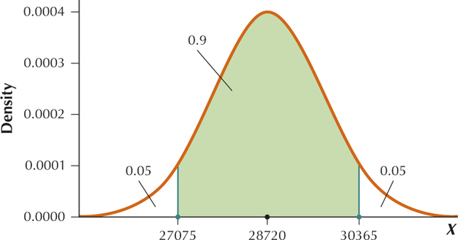
YOUR TURN #5
Section 7.1, page 407
From Example 7, and . We want the middle 90% of the sample means, so we will use our calculators to find the sample mean with 5% to the left of it and the sample mean with 95% to the left of it. The calculator gives us mpg and mpg.

A-13
YOUR TURN #6
Section 7.2, page 415
The survey sample size is , and the number of successes is . We calculate
YOUR TURN #7
Section 7.2, page 416
From Example 11, . . Then and .
YOUR TURN #8
Section 7.2, page 420
We want to find . From Example 13, . From Example 13 (a) the minimum sample size required to produce a sampling distribution of that is approximately normal is 117 vehicles. Since vehicles is greater than 117 vehicles, the sampling distribution of is approximately normal. Then and
Notice from the graph that if we use technology to find
We standardize as follows:
Then .
YOUR TURN #9
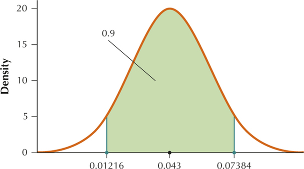
Section 7.2, page 421
From Example 13, and . The middle 90% lies between the 5th and the 95th percentile. Using the calculator we get the 5th percentile ≈ 0.01216 and the 95th percentile ≈ 0.07384. Therefore the middle 90% lies between 0.01216 and 0.07384.
Chapter 8
YOUR TURN #1
Section 8.1, page 429
(a) The sample mean yield is calculated as
(b) The point estimate of μ, the unknown nationwide mean winter wheat yield for all 50 states, is 60.4 bushels per acre.
YOUR TURN #2
Section 8.1, page 431
- (a) Since the population is not normally distributed and the sample size is less than 30, the interval may not be used.
- (b) Since the sample size is greater than or equal to 30 and σ is known, the interval may be used.
YOUR TURN #3
Section 8.1, page 432
- (a) Table 1 gives us .
- (b) Table 1 gives us .
YOUR TURN #4
Section 8.1, page 433
Because the population is normal and the population standard deviation σ is known, the requirements for the interval are met:
We are given , and . From Table 1, we have . Thus,
Thus we are 95% confident that the population mean score on the 2014 Mathematics SAT test lies between 463.74 and 556.26.
YOUR TURN #5
Section 8.1, page 434
The formula for the confidence interval is given by
We are given , and . From Table 1, we have . Plugging into the formula:
We are 99% confident that μ, the population mean city MPG for all motor vehicles, lies between 19.26 mpg and 22.16 mpg.
A-14
YOUR TURN #6
Section 8.1, page 441
“Within $100” means that the margin of error is $100, and 1.96 is the value associated with 95% confidence. Substituting into the formula for sample size we get:
YOUR TURN #7
Section 8.2, page 451
First we need to find our degrees of freedom, . Then, using the table for a 90% confidence interval, .
YOUR TURN #8
Section 8.2, page 452
- (a) The sample size is not large ( is not ≥ 30) and we are not told that the population is normal. Therefore, the conditions are not met for the interval for μ. It is not okay to construct the interval.
- (b) We are not told that the population is normal. However, the sample size is large ( is ≥ 30). Therefore, the conditions are met for the interval for μ. It is okay to construct the interval.
YOUR TURN #9
Section 8.2, page 453
The value of for 95% confidence and 15 degrees of freedom is 2.131. A 95% confidence interval for μ is given by the interval
From Example 14, , and , From the table, . Substituting, we get
We are 95% confident that μ, the population mean sodium content per serving of all breakfast cereals, lies between 155.6 grams and 216.2 grams.
YOUR TURN #10
Section 8.2, page 454
From Your Turn #9, we have:
The margin of error for mean sodium content is 30.3 grams. We can estimate the population mean sodium content per serving of all breakfast cereals to within 30.3 grams with 95% confidence.
YOUR TURN #11
Section 8.3, page 463
(a)
The point estimate of the proportion is 0.5.
(b)
The point estimate of the proportion is 0.5625.
YOUR TURN #12
Section 8.3, page 465
(a) There are successes, which is ≥ 5 and there are failures, which is also ≥ 5. The conditions for constructing the interval for have been met.
From Table 1, the confidence level of 95% gives . Thus, the confidence interval is
We are 95% confident that the population proportion lies between 0.402 and 0.598.
(b) There are successes, which is ≥ 5 and there are failures, which is also ≥ 5. The conditions for constructing the interval for have been met.
From Table 1, the confidence level of 95% gives . Thus, the confidence interval is
We are 95% confident that the population proportion lies between 0.4856 and 0.6394.
YOUR TURN #13
Section 8.3, page 467
(a) The margin of error is
We can estimate the population proportion to within 0.098 with 95% confidence.
(b) The margin of error is
We can estimate the population proportion to within 0.0769 with 95% confidence.
YOUR TURN #14
Section 8.3, page 469
The required sample size is
Rounding up, this gives us a minimum required sample size of 1719.
YOUR TURN #15
Section 8.3, page 469
The required sample size is
Rounding up, this gives us a minimum required sample size of 385.
YOUR TURN #16
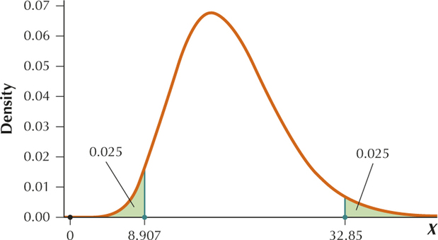
Section 8.4, page 476
For a 95% confidence interval,
A-15
So we are seeking , the critical value with area to the right of it and the critical value with area to the right of it. Because , the degrees of freedom is . From the table, .
Chapter 9
YOUR TURN #1
Section 9.1, page 492
Step 1 Search the word problem for certain key English words and select the appropriate symbol.
The problem uses the word “increased” which means “is greater than.” Thus, we will use a hypothesis that contains the > symbol.
Step 2 Determine the form of the hypothesis.
From Table 1, we see that the > symbol means that we use a right-tail test:
Step 3 Find the value for and write your hypotheses.
The alternative hypothesis states that the mean monthly amount of time that iPhone and Android users spend using the apps on their devices has increased from some value . Increased from what? 30 hours per month. Write the two hypotheses with .
YOUR TURN #2
Section 9.1, page 495
(a) A Type I error would be to reject when is true. This would be to conclude that μ is less than 7 when, in reality, . In other words, a Type I error would be to conclude that the population mean of the pair of dice tossed in Example 1 is less than 7 when, in reality, it is equal to 7.
A Type II error occurs when we do not reject when is false. This would be to conclude that μ is equal to 7 when, in reality, it is less than 7.
(b) A Type I error would be to reject when is true. This would be to conclude that μ had decreased when, in reality, it had stayed the same. In other words, a Type I error would be to conclude that the population mean rainfall in Arizona had decreased when, in reality, it had not decreased.
A Type II error occurs when we do not reject when is false. This would be to conclude that μ had stayed the same when, in reality, it had decreased.
YOUR TURN #3
Section 9.2, page 499
Now , but have all stayed the same.
Therefore,
YOUR TURN #4
Section 9.2, page 501
- (a) We have a right-tailed test and level of significance , so Table 4 tells us that the critical value is .
- (b)
YOUR TURN #5
Section 9.3, page 509
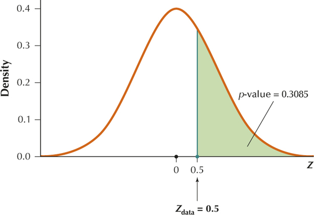
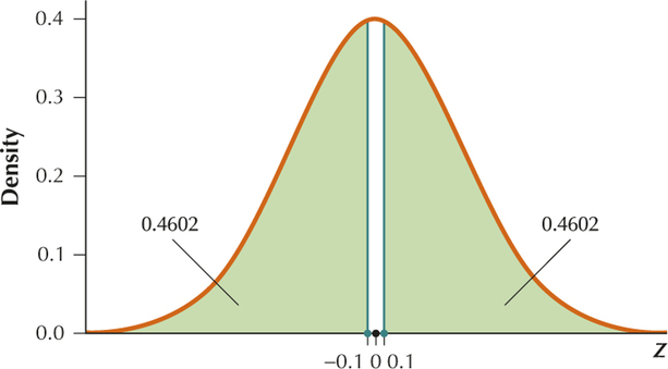
(a) We have a right-tailed test, so that the -value is the area in the right tail:
The table gives the probability for . Thus,
(b) We have a left-tailed test, so that the -value is the area in the left tail:
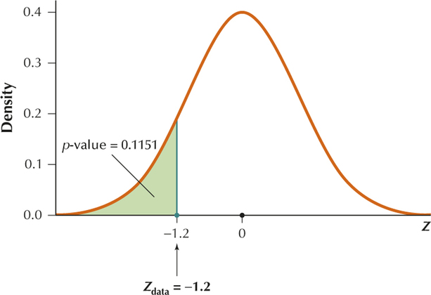
A-16
(c) Here, we have a two-tailed test, so that the -value is the sum of the area in the two tails:
YOUR TURN #6
Section 9.3, page 515
- (a) The -value of 0.1587 implies that there is no evidence against the null hypothesis that the population mean equals 3.0.
- (b) The -value of 0.0735 implies that there is moderate evidence against the null hypothesis that the population mean equals 10.
- (c) The -value of 0.0456 implies that there is solid evidence against the null hypothesis that the population mean equals 100.
YOUR TURN #7
Section 9.3, page 518
| Value of |
Form of hypothesis test, with |
Where lies in relation to 90% confidence interval |
Conclusion of hypothesis test |
|---|---|---|---|
| a. 548 | Inside | Do not reject | |
| b. 477 | Inside | Do not reject | |
| a. 549 | Outside | Reject |
YOUR TURN #8
Section 9.4, page 528
(a) Step 1 State the hypotheses.
From Example 18 the hypotheses are
where refers to the population mean age at onset.
Step 2 Find and state the rejection rule.
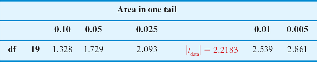
We still have a left-tailed test and df = 19, but now . From the table . Therefore we will reject if .
Step 3 Calculate .
From Example 18 .
Step 4 State the conclusion and interpretation.
The rejection rule from Step 2 says to reject if . From Step 3, we have . Because −2.2183 is not less than −2.539, our conclusion is to not reject . There is insufficient evidence at level of significance that the population mean age of onset has decreased from its previous level of 15 years.
(b) In Example 18, and the conclusion is to reject . In (a), and the conclusion is to not reject . This is because the cutoff for rejecting the null hypothesis at the cutoff for rejecting the null hypothesis at .
From the “Developing Your Statistical Sense” box on p. 515, there are two alternatives available in situations like this.
- Turn to a direct assessment of the strength of evidence against the null hypothesis.
- Obtain more data, perhaps through a call for further research.
YOUR TURN #9
Section 9.4, page 531
- (a) The hypotheses do not depend on α. Therefore, a change in α will not affect the hypotheses.
- (b) The test statistic does not depend on α. Therefore, a change in α will not affect .
- (c) The -value does not depend on α. Therefore, a change in α will not affect the -value.
- (d) The conclusion does depend on α. Decreasing α from to changes the rejection rule from reject if the to reject if the . The is not ≤ 0.01. Therefore we do not reject . Thus the conclusion has changed from reject if to do not reject if .
YOUR TURN #10
Section 9.4, page 534
From Example 18, our hypotheses are
Our test statistic is and df = 19.
We have a left-tailed test, which is a one-tailed test. Since the table only has positive values of , we will look up in the table.
From the table we see that . Therefore .
YOUR TURN #11
Section 9.5, page 544
The sample proportion of Chromebooks is
We then calculate the value of the test statistic :
YOUR TURN #12
Section 9.5, page 548
Step 1 State the hypotheses and the rejection rule.
The hypotheses are
where represents the population proportion of young people ages 18–24 who had an accident. We reject if the -value .
Step 2 Calculate .
Our sample proportion is .
A-17
Thus, our test statistic is
Step 3 Find the -value.
We have a right-tailed test, so the -value is
Step 4 State the conclusion and the interpretation.
The -value 0.0018 is , so we reject . There is evidence that the population proportion of young people ages 18–24 who had an accident has increased.
Chapter 10
YOUR TURN #1
Section 10.1, page 578
For each student, we subtract the “Before” value from the “After” value.
We now consider the set of these six differences {−2, 0, 1, 1, 2, 4} as a sample.
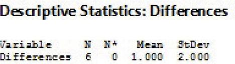
From the Minitab output we see that .
YOUR TURN #2
Section 10.1, page 580
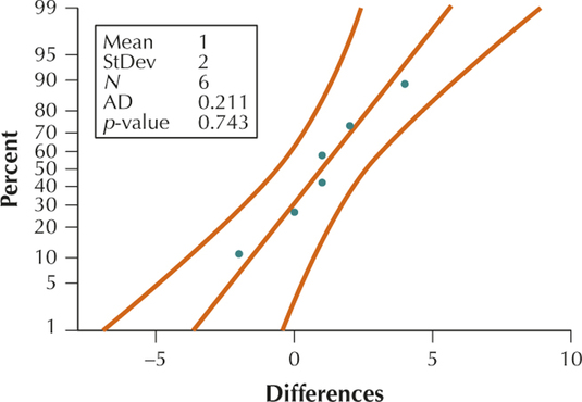
From the normal probability plot we see that we have acceptable normality.
Step 1 State the hypotheses.
The hypotheses are
where represents the population mean difference in English quiz scores.
Step 2 Find the critical value and state the rejection rule.
We have a right-tailed test with area in one tail equal to and degrees of freedom equal to . Therefore our critical value from the table is . Therefore our rejection rule is that we will reject when is greater than or equal to 1.476.
Step 3 Find .
From Your Turn #1, . Therefore
Step 4 State the conclusion and the interpretation.
Since is not greater than or equal to 1.476, we do not reject . There is insufficient evidence at level of significance that the population mean difference of English quiz scores is greater than 0.
YOUR TURN #3
Section 10.1, page 583
The normality was checked in Your Turn #2. From Your Turn #1, and . For a 90% confidence interval with degrees of freedom equal to .
Using these values,
We are 90% confident that the population mean of the differences between English quiz scores before and after visiting the English Center lies between −0.6452 point and 2.6452 points.
YOUR TURN #4
Section 10.1, page 584
From Your Turn #3, our 90% confidence interval is (−0.6452, 2.6432).
(a)
lies inside the interval, so we do not reject .
(b)
lies outside the interval, so we reject .
(c)
lies outside the interval, so we reject .
Chapter 11
YOUR TURN #1
Section 11.1, page 634
(a) There are possible outcomes: paperbacks, hardcovers, e-Books, and all other formats. Assigning probabilities using the relative frequency method, we have the following hypothesized proportions for each book format:
and
Therefore, = book format is a valid multinomial random variable.
(b) We have books (sample size = 2000), so the expected frequencies are as provided in the following table.
Category Paperback Hardcover e-Book All other formats
A-18
YOUR TURN #2
Section 11.1, page 637
| Category | ||||||
|---|---|---|---|---|---|---|
| Paperback | 0.41 | 810 | 820 | −10 | 100 | |
| Hardcover | 0.34 | 680 | 680 | 0 | 0 | |
| e-Book | 0.13 | 280 | 260 | 20 | 400 | |
| All other formats |
0.12 | 230 | 240 | −10 | 100 |
Then
YOUR TURN #3
Section 11.1, page 638
Step 1 State the hypotheses and check the conditions. The hypotheses are:
: The random variable does not follow the distribution specified in .
Checking the conditions, the expected frequencies from Your Turn #1 are
Because none of these expected frequencies is less than one, and none of the expected frequencies is less than five, the conditions for performing the goodness of fit test are met.
Step 2 Find the critical value, and state the rejection rule.
We have degrees of freedom and Then, from the table, . The rejection rule is “Reject if .”
Step 3 Find .
From Your Turn #2,
Step 4 State the conclusion and interpretation.
Compare with is not . Therefore, we do not reject . There is insufficient evidence that the variable book format does not follow the distribution specified in . In other words, there is insufficient evidence that the book format market shares have changed.
Chapter 12
There are no Your Turn exercises in this chapter.
Chapter 13
YOUR TURN #1
Section 13.1, page 717
(a)
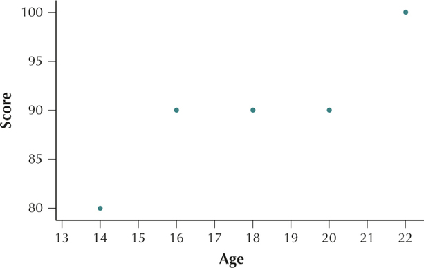
As age increases, the score on the video game tends to increase.
- (b) As calculated by the TI-84, . Age and score are positively correlated. An increase in age is associated with an increase in the score on the video game.
- (c) As calculated by the TI-84, . The slope means there is an estimated increase of 2 in the score on the video game for each one year increase in age. The -intercept is the estimated score on the video game of someone aged .
(d) For a 22-year-old person, the estimated score on the video game is .
The actual score of the 22-year-old person in the sample is . Thus, our prediction error is . The 22-year-old person scored slightly higher than expected.
YOUR TURN #2
Section 13.1, page 721
(a)
= score on
video gameFitted (predicted)
values
Residuals 14 80 82 −2 16 90 86 4 18 90 90 0 20 90 94 −4 22 100 98 2 (b)
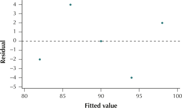
The scatterplot of the residuals versus the fitted values shows no evidence of the unhealthy patterns shown in Figure 4. Thus, the independence assumption, the constant variance assumption, and the zero-mean assumption are verified.
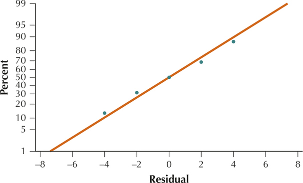
Also, the normal probability plot of the residuals indicates no evidence of departures from normality in the residuals. Therefore, we conclude that the regression assumptions are verified.
YOUR TURN #3
Section 13.1, page 725
Hypothesis test using the -value method.
Step 1 State the hypotheses and the rejection rule.
No linear relationship exists between age and score.
A linear relationship exists between age and score.
Reject if the .
A-19
Step 2 Calculate .
From Your Turn #1, . From the TI-84, . Therefore,
. The residuals were calculated in Your Turn #2 (a). They are −2, 4, 0, −4, and 2. Therefore,
Thus
Step 3 Find the -value.
Using the TI-84 we get .
Step 4 State the conclusion and the interpretation.
The -value = 0.0405193264 is , so we reject . Evidence exists, at level of significance , for a linear relationship between age and score.
Hypothesis test using the critical value method.
Step 1 State the hypotheses No linear relationship exists between age and score.
A linear relationship exists between age and score.
Step 2 Find the critical value and the rejection rule.
The degrees of freedom are . We have a two-tailed test with . From the table, . Therefore the rejection rule is Reject if .
Step 3 Calculate .
From Your Turn #1, . From the TI-84, . Therefore,
. The residuals were calculated in Your Turn #2 (a). They are −2, 4, 0, −4, and 2. Therefore,
Thus
Step 4 State the conclusion and the interpretation.
is ≥ 3.182, so we reject . Evidence exists, at level of significance , for a linear relationship between age and score.
A-20