9.4 Test for the Population Mean
525
OBJECTIVES By the end of this section, I will be able to …
- Perform the test for the mean using the critical-value method.
- Perform the test for the mean using the -value method.
- Use confidence intervals to perform two-tailed hypothesis tests.
1 Test for Using the Critical-Value Method
Note: Students may want to review the characteristics of the distribution on page 450 of Chapter 8.
In many real-world scenarios, the value of the population standard deviation is unknown. When this occurs, we should use neither the interval nor the test. Recall that in Section 8.2, we used the distribution to find a confidence interval for the mean when σ was not known. The situation is similar for hypothesis testing.
Let be the sample mean, be the unknown population mean, be the sample standard deviation, and be the sample size. The t statistic
with degrees of freedom may be used when either the population is normal or the sample size is large. We call this statistic because its value depends largely on the sample data.
The test statistic used for the test for the mean is
represents the number of standard errors lies above or below .
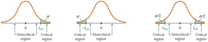
Extreme values of , that is, values of that are significantly far from the hypothesized , will translate into extreme values of . In other words, just as with , when is far from , will be far from 0. We answer the question “How extreme is extreme?” using the critical-value method by finding a critical value of t, called . This threshold value separates the values of for which we reject (the critical region) from the values of for which we will not reject (the noncritical region). Because a different curve exists for every different sample size, you need to know the following to find the value of : (a) the form of the hypothesis test (right-tailed, left-tailed, or two-tailed), (b) the degrees of freedom , and (c) the level of significance .
The degrees of freedom is a measure of how the distribution changes as the sample size changes.
Test for the Population Mean : Critical-Value Method
When a random sample of size is taken from a population, you can use the test if either the population is normal or the sample size is large .
Step 1 State the hypotheses.
Use one of the forms from Table 8. State the meaning of .
Step 2 Find and state the rejection rule.
Use Table D in the Appendix and Table 8.
Step 3 Calculate .
Step 4 State the conclusion and the interpretation.
If falls within the critical region, then reject . Otherwise, do not reject . Interpret your conclusion so that a nonspecialist can understand.
526
| Form of test | Right-tailed test | Left-tailed test | Two - tailed test |
|---|---|---|---|
| Hypotheses |
level of significance |
level of significanc |
level of significance |
| Critical region |
|
||
| Rejection rule | Reject if | Reject if | Reject if or |
EXAMPLE 18 Test for using critical-value method: Left-tailed test
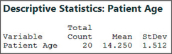
We are interested in testing, using level of significance , whether the mean age at onset of anorexia nervosa in young women has been decreasing. Assume that the previous mean age at onset was 15 years old. Data were gathered for a study of the onset age for this disorder.6 From these data, a random sample (shown here) was taken of young women who were admitted under this diagnosis to the Toronto Hospital for Sick Children. The Minitab descriptive statistics shown here indicate a sample mean age of years and a sample standard deviation of years. If appropriate, perform the test.
| 14.50 | 15.75 | 14.17 | 14.00 |
| 14.67 | 17.25 | 11.00 | 16.00 |
| 14.50 | 15.17 | 12.00 | 13.00 |
| 13.00 | 13.50 | 15.42 | 16.08 |
| 14.00 | 12.58 | 13.50 | 14.92 |
Solution
The sample size is not large, so we need to verify normality. The normal probability plot of the ages at onset in Figure 18 indicates that the ages in the sample are normally distributed. We may proceed to perform the test for the mean.
Step 1 State the hypotheses.
The key word “decreasing” guides us to state our hypotheses as follows:
where refers to the population mean age at onset.
Step 2 Find and state the rejection rule.
Our hypotheses from Step 1 indicate that we have a left-tailed test, meaning that the critical region represents an area in the left tail (see Figure 20, page 528). To find , we turn to the table, an excerpt of which is shown in Figure 19. Because we have a one-tailed test, under “Area in one tail,” select the column with our value 0.05. Then choose the row with our , so that we get . Because we have a left-tailed test, the rejection rule from Table 8 is “Reject if ”; that is, we will reject if .
527
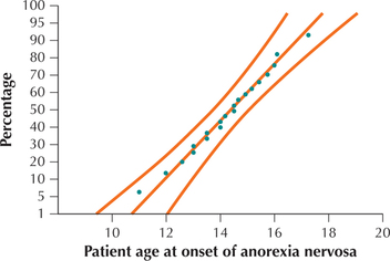 Figure 9.23: FIGURE 18 Normal probability plot for age at onset of anorexia nervosa.
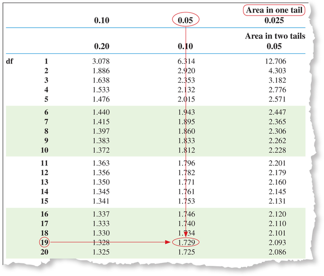 Figure 9.24: FIGURE 19 Finding for a one-tailed test. For a two-tailed test, use “Area in two tails.”
Step 3 Calculate .
We have , , and . Also, , because this is the hypothesized value of stated in . Therefore, our test statistic is
Step 4 State the conclusion and interpretation.
The rejection rule from Step 2 says to reject if . From Step 3, we have . Because −2.2183 is less than −1.729, our conclusion is to reject . If you prefer the graphical approach, consider Figure 20, which shows where falls in relation to the critical region. Because falls within the critical region, our conclusion is to reject . There is evidence at level of significance that the population mean age of onset has decreased from its previous level of 15 years.
528
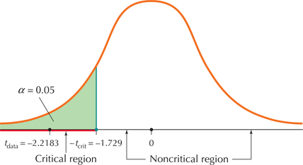 Figure 9.25: FIGURE 20 Our falls in the critical region.
NOW YOU CAN DO
Exercises 3–8.
YOUR TURN #8
- For the data in Example 18, test, using level of significance , whether the mean age at onset of anorexia nervosa in young women has been decreasing.
- Discuss two possible resolutions to the contradiction between the conclusions in Example 18 and Part (a).
(The solutions are shown in Appendix A.)
EXAMPLE 19 Test for using critical-value method: two-tailed test
CNN reported in 2014 that, even after factoring in part-time jobs, Americans worked an average of 38 hours per week. Suppose a social science researcher disputes this finding and is interested in testing whether the population mean number of hours worked per week differs from 38. A random sample of working Americans yields a sample mean of hours worked, with a sample standard deviation of hours. If the conditions are met, perform the appropriate hypothesis test using level of significance .
Solution
Because , we may proceed with the test.
Step 1 State the hypotheses.
The key words “differs from” indicate a two-tailed test, with , because we are testing whether differs from 38. So our hypotheses are
where represents the population mean number of hours worked per week.
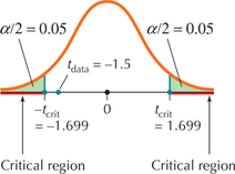 Figure 9.26: FIGURE 21 Critical region for two-tailed test.
Step 2 Find and state the rejection rule.
To find for a two-tailed test with level of significance , we look in the 0.10 column in the “Area in two tails” section of Table D in the Appendix. The degrees of freedom gives us . From Table 8, the rejection rule is: “Reject if or .”
529
Step 3 Calculate :
Step 4 State the conclusion and the interpretation.
is not ≥1.699 and it is not ≤−1.699; therefore, we do not reject . See Figure 21. There is insufficient evidence, at level of significance , that the population mean number of hours worked per week differs from 38.
NOW YOU CAN DO
Exercises 9–14.
2 Test for Using the -Value Method
We may also use the -value method for performing the test for . The critical-value method and the -value are equivalent, so they will provide identical conclusions.
t Test for the Population Mean : -Value Method
When a random sample of size is taken from a population, you can use the test if either the population is normal or the sample size is large .
Step 1 State the hypotheses and the rejection rule.
Use one of the forms from Table 9. State the meaning of . The rejection rule is “Reject if the .”
Step 2 Calculate .
Step 3 Find the -value.
Either use technology to find the -value or estimate the -value using Table D, Distribution, in the Appendix.
Step 4 State the conclusion and the interpretation.
If the , then reject . Otherwise, do not reject . Interpret your conclusion.
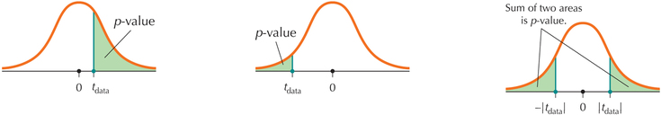
The definition of a -value for a test is similar to the -value for a test. Unusual and extreme values of , and therefore of , will have a small -value, whereas values of and nearer to the center of the distribution will have a large -value. Table 9 summarizes the definition of the -value for tests. Note that we will not be finding these -values manually but will either (a) use a computer or calculator or (b) estimate them using the table.
| Form of test | Right-tailed test | Left-tailed test | Two-tailed test |
|---|---|---|---|
| Hypotheses | |||
|
-Value = is tail area associated with |
|||
|
|||
530
EXAMPLE 20 Test using the -value method: Right-tailed test
milkprice
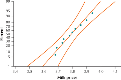
The U.S. Bureau of Labor Statistics reports that the mean price for a gallon of milk in July 2014 was $3.65. Gallons of milk were recently bought in a random sample of different cities, with the prices shown in the accompanying table. Test, using level of significance , whether the population mean price for a gallon of milk is greater than $3.65.
Solution
We first check whether the conditions for performing the test are met. Because our sample size is small, we must check for normality. The normal probability plot in Figure 22 shows acceptable normality, allowing us to proceed with the test.
Step 1 State the hypotheses and the rejection rule.
The key words “is greater than” means that we have a right-tailed test. Answering the question “Greater than what?” gives us .
where represents the population mean price of milk. We will reject if the .
Step 2 Calculate .
We use the instructions from the Step-by-Step Technology Guide on page 537. Figure 23 shows the TI-83/84 results from the test for .
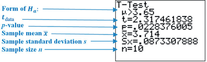 Figure 9.28: FIGURE 23 TI-83/84 results for right-tailed test.
For a more accurate calculation of the -value, we retain 9 decimal places for the value of .
Using the statistics from Figure 23, we have the test statistic
Step 3 Find the -value.
From Figures 23 and 24, we have
531
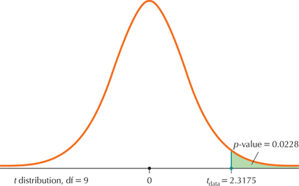 Figure 9.29: FIGURE 24 The -value for a right-tailed test.
Step 4 State the conclusion and the interpretation.
The is less than the level of significance ; therefore, reject . There is evidence, at level of significance , that the population mean price of milk is greater than $3.65.
NOW YOU CAN DO
Exercises 15–20.
YOUR TURN #9
In Example 20, suppose the level of significance was . Describe how this would affect the following, if at all:
- Hypotheses
- -value
- Conclusion
(The solutions are given in Appendix A.)
EXAMPLE 21 Test using the -value method: Two-tailed test
The Golden Ratio
Euclid's Elements, the Parthenon, the Mona Lisa, and the beadwork of the Shoshone tribe all have in common an appreciation for the golden ratio.
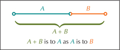
Suppose we have two quantities and , with . Then is called the golden ratio if
that is, if the ratio of the sum of the quantities to the larger quantity equals the ratio of the larger to the smaller (see Figure 25a).
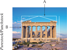
Euclid wrote about the golden ratio in his Elements, calling it the “extreme and mean ratio.” The ratio of the width and height of the Parthenon, one of the most famous temples in ancient Greece, equals the golden ratio (Figure 25b). If you enclose the face of Leonardo da Vinci's Mona Lisa in a rectangle, the resulting ratio of the long side to the short side follows the golden ratio (Figure 26). The golden ratio has a value of approximately 1.618.
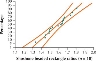
Now, we will test whether evidence exists for the use of the golden ratio in the artistic traditions of the Shoshone, a Native American tribe from the American West. Figure 27 shows a detail of a nineteenth-century Shoshone beaded dress that belonged to Nahtoma, the daughter of Chief Washakie of the Eastern Shoshone.7 It is intriguing to consider whether the Shoshone beaded rectangles, such as those on this dress, follow the golden ratio. Table 10 contains the ratios of lengths to widths of 18 beaded rectangles made by Shoshone artisans.8 We will perform a hypothesis test to determine whether the population mean ratio of Shoshone beaded rectangles equals the golden ratio of 1.618.
532


shoshone
| 1.44 | 1.75 | 1.64 | 1.66 | 1.64 |
| 1.51 | 1.34 | 1.53 | 1.74 | 1.81 |
| 1.45 | 1.49 | 1.63 | 1.49 | |
| 1.65 | 1.59 | 1.50 | 1.65 |
Solution
The population standard deviation for such rectangles is unknown, so we must use a test instead of a test. Our sample size is not large, so we must assess whether the data are normally distributed. Figure 28 shows the normal probability plot, indicating acceptable support for the normality assumption. We proceed with the test, using level of significance .
We use the TI-83/84 and CrunchIt! to perform this hypothesis test, using the Step-by-Step Technology Guide at the end of this section.
Step 1 State the hypotheses and the rejection rule.
We are interested in whether the population mean length-to-width ratio of Shoshone beaded rectangles equals the golden ratio of 1.618, so we perform a two-tailed test:
where represents the population mean length-to-width ratio of Shoshone beaded rectangles. We will reject if the .
533
Step 2 Find .
Using the statistics from Figure 29a, we have the test statistic
Step 3 Find the -value.
From Figures 29a, 29b, and 30, we have
Step 4 State the conclusion and interpretation.
Because is , we do not reject . Thus, there is insufficient evidence, at level of significance , that the population mean ratio differs from 1.618. In other words, the data do not reject the claim that Shoshone beaded rectangles follow the same golden ratio exhibited by the Parthenon and the Mona Lisa.
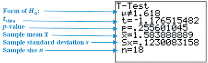 Figure 9.35: FIGURE 29a TI-83/84 results.
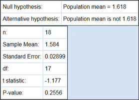 Figure 9.36: FIGURE 29b CrunchIt! results.
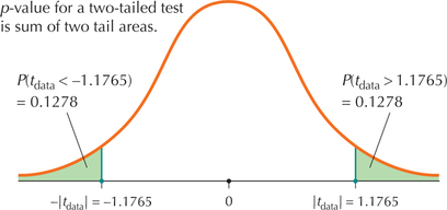 Figure 9.37: FIGURE 30 -Value for two-tailed test is sum of two tail areas.
NOW YOU CAN DO
Exercises 21–26.
EXAMPLE 22 Estimating the -value using the table
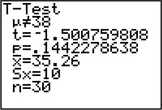
Suppose we did not have access to technology. Estimate the -value from Example 19 using the table (Appendix Table D). For Example 19, our hypotheses are
where represents the population mean number of hours worked per week. Our test statistic is .
Solution
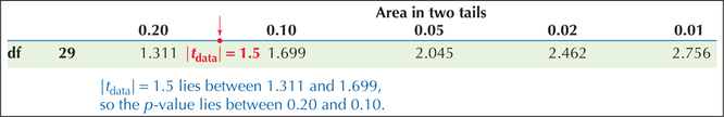
For a two-tailed test, choose the row of the table with the heading “Area in two tails.” Then select the row in the table with the appropriate degrees of freedom, in this case . Note the -values in this row: 1.311, 1.699, 2.045, 2.462, and 2.756. Think of these values as existing on a horizontal number line. We want to place our somewhere on this number line, but all the -values in the table are positive. Fortunately, because of the symmetry of the distribution about zero, we may take . Now, where would fit on this “number line”? Between 1.311 and 1.699, as indicated in Figure 31, an excerpt from the table. Therefore, we may estimate the -value to be between 0.20 and 0.10. In fact, the actual -value for this problem is about 0.144 (see Figure 32), so that our estimate is confirmed.
534
NOW YOU CAN DO
Exercises 27–30.
YOUR TURN #10
Estimate the -value for the hypothesis test in Example 18.
(The solution is shown in Appendix A.)
3 Using Confidence Intervals to Perform Two-Tailed tests
Just as we did for two-tailed tests in Section 9.3, we may use a confidence interval to perform a two-tailed test with level of significance for various hypothesized values of . The strategy is the same: if a certain value for lies outside the confidence interval for , then the null hypothesis specifying this value for would be rejected. Otherwise, it would not be rejected.
EXAMPLE 23 Using a confidence interval to perform two-tailed tests
In Example 14 of Chapter 8 (page 452), we found the 99% -confidence interval for , the population mean sodium content per serving of all breakfast cereals, to be the following:
Test, using level of significance , whether the population mean amount of sodium differs from the following values: (a) 100 grams, (b) 170 grams, (c) 250 grams.
Solution
The key words “differs from” mean that we are using two-tailed tests. Then, for each hypothesized value of , we determine whether it falls inside or outside the given confidence interval.
-
The confidence interval is (144.1, 227.7), and because lies outside the interval (see Figure 33), we reject .
535
lies inside the interval, so we do not reject .
lies outside the interval, so we reject .
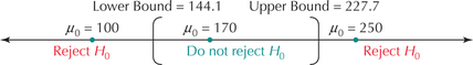 Figure 9.40: FIGURE 33 Reject for values of that lie outside (144.1, 227.7).
NOW YOU CAN DO
Exercises 31–36.
In Section 9.3, we showed how to perform and interpret tests for using the TI-83/84 and Minitab software output. Here, in Section 9.4, we demonstrate how to perform and interpret tests for using software output from SPSS and JMP.
EXAMPLE 24 Interpreting software output
Each of (a) and (b) represent software output from a test for . For each, examine the indicated software output, and provide the following steps:
- Step 1 State the hypotheses and the rejection rule.
- Step 2 Find .
- Step 3 Find the -value.
- Step 4 State the conclusion and the interpretation.
Use level of significance for each hypothesis test.
SPSS output for a test for , where represents the population mean number of orchard farms per county, nationwide.
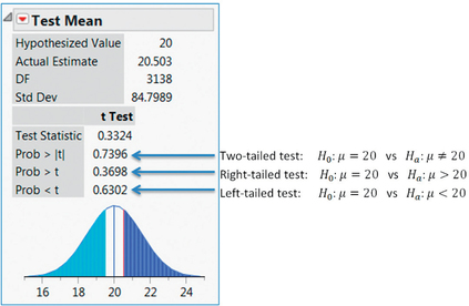
JMP output for a test for , where represents the population mean number of grocery stores per county, nationwide.
536
Solution
- Interpreting the SPSS output.
Step 1 State the hypotheses and the rejection rule.
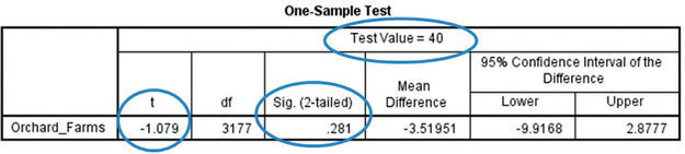
In the SPSS output, the “Test ” indicates that . Also, the “2-tailed” in the output indicates that we have a two-tailed test. Thus, our hypotheses are:
where represents the population mean number of orchard farms per county, nationwide. We will reject if the -value is less than level of significance .
Step 2 Find .
Under the “t” in the SPSS is the value for .
Step 3 Find the -value.
The abbreviation “Sig.” stands for “Significance,” which represents the -value: 0.281.
Step 4 State the conclusion and the interpretation.
The -value of 0.281 is not less than the level of significance , so we do not reject . There is insufficient evidence that the population mean number of orchard farms per county differs from 40.
- Interpreting the JMP output.
Step 1 State the hypotheses and the rejection rule.
In the JMP output, the “Hypothesized Value” indicates that . Now, JMP is unusual in that it performs all three types of hypothesis test simultaneously: two-tailed, right-tailed, and left-tailed, as shown in the JMP output. It does not specify a particular form of the test. Let us use the right-tailed test for this example. Thus, our hypotheses are:
where represents the population mean number of grocery stores per county, nationwide. We will reject if the -value is less than level of significance .
Step 2 Find .
Next to “Test Statistic” in the JMP output, we find the value of our test statistic, , 0.3324.
Step 3 Find the -value.
Here, we need to be careful, because JMP gives us three different -values, depending on which form of the hypothesis test is performed. We chose the right-tailed test, so our -value is next to , as indicated in the JMP output.
Step 4 State the conclusion and the interpretation.
The -value of 0.3698 is not less than the level of significance , so we do not reject . There is insufficient evidence that the population mean number of grocery stores per county is greater than 20.
NOW YOU CAN DO
Exercises 37–40.