9.5 Test for the Population Proportion
543
OBJECTIVES By the end of this section, I will be able to …
- Perform the test for using the critical-value method.
- Perform the test for using the -value method.
- Use confidence intervals for to perform two-tailed hypothesis tests about .
1 The Test for Using the Critical-Value Method
For example, if a baseball player has hits in at-bats, his batting average is (or .300).
Thus far, we have dealt with testing hypotheses about the population mean only. In this section, we will learn how to perform the test for the population proportion . For our point estimate of the unknown population proportion , we use the sample proportion , where equals the number of successes.
Just as with the test for the mean, in the test for the proportion the null hypothesis will include a certain hypothesized value for the unknown parameter, which we call . For example, the hypotheses for the two-tailed test have the following form:
where represents a particular hypothesized value of the unknown population proportion . For instance, if a researcher is interested in determining whether the population proportion of Americans who support increased funding for higher education differs from 50%, then and .
If we assume is correct, then the population proportion of successes is Then Facts 5 and 6 from Section 7.2 tell us that the sampling distribution of has a mean of and the standard deviation
because we claim in that Here, is called the standard error of the proportion. Fact 7 from Section 7.2 tells us that the sampling distribution of is approximately normal whenever both of the following conditions are met: and . This leads us to the following statement of the essential idea about hypothesis testing for the proportion.
The essential idea About Hypothesis testing for the Proportion
When the sample proportion is unusual or extreme in the sampling distribution of that is based on the assumption that is correct, we reject . Otherwise, there is insufficient evidence against , and we should not reject .
The remainder of this section explains the details of implementing hypothesis testing for the proportion. The critical-value method for the test for is similar to that of the test for , in that we compare one -value () with another -value (). In this section, represents the number of standard errors () the sample proportion lies above or below the hypothesized proportion .
The test statistic used for the test for the proportion is
where is the observed sample proportion of successes, is the value of hypothesized in , , and is the sample size.
544
EXAMPLE 25 Calculating for the test for proportion
The NPD Group reported in 2013 that sales of the Chromebook accounted for 20% of the U.S. computer market. Suppose a random sample of computers found 76 that were Chromebooks. We are interested in testing whether the population proportion of Chromebooks has changed from 20%.
- Construct the hypotheses.
- Calculate the test statistic .
Solution
The key words “has changed” indicate a two-tailed test. “Changed from what?” The hypothesized proportion . The hypotheses are
The sample proportion of Chromebooks is
We then calculate the value of the test statistic :
NOW YOU CAN DO
Exercises 7–14.
YOUR TURN #11
For Example 25, suppose the sample found 50 of 400 computers that were Chromebooks. Calculate the test statistic .
(The solution is shown in Appendix A.)
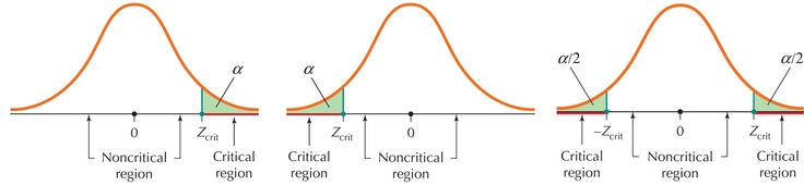
To find the critical values, the critical regions, or the rejection rules, you can use Table 11.
| Form of Hypothesis Test | |||
|---|---|---|---|
| Level of significance |
Right-tailed |
Left-tailed |
Two-tailed |
| 0.10 | |||
| 0.05 | |||
| 0.01 | |||
|
|||
| Rejection rule | Reject if |
Reject if |
Reject if or |
545
test for the Population Proportion : Critical-value Method
When a random sample of size is taken from a population, you can use the test for the proportion if both of the normality conditions are satisfied:
Step 1 State the hypotheses.
Use one of the forms from Table 11. State the meaning of .
Step 2 Find and state the rejection rule.
Use Table 11.
Step 3 Calculate .
Step 4 State the conclusion and the interpretation.
If falls in the critical region, then reject . Otherwise, do not reject . Interpret the conclusion so that a nonspecialist can understand.
EXAMPLE 26 test for using the critical-value method
As a check on your arithmetic, the two quantities you obtain when checking the normality conditions should add up to . Here, .
Refer to Example 25. Test whether the population proportion of Chromebook computers has changed from 20%, using the critical-value method and level of significance .
Solution
First, we check that both of our normality conditions are met. From Example 25, we have and .
The normality conditions are met and we may proceed with the hypothesis test.
Step 1 State the hypotheses.
From Example 25, our hypotheses are
where represents the population proportion of computers that are Chromebooks.
Step 2 Find and state the rejection rule.
We have a two-tailed test, with . This gives us our critical value . the rejection rule from Table 11 is: Reject if or (Figure 35).
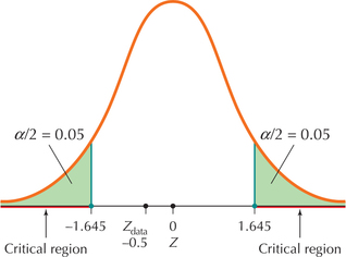 Figure 9.45: FIGURE 35 does not fall in the critical region.
Step 3 Calculate .
From Example 25, we have
546
Step 4 State the conclusion and the interpretation.
The test statistic is not and not . Thus, we do not reject . There is insufficient evidence at level of significance that the population proportion of computers that are Chromebooks differs from 20%.
NOW YOU CAN DO
Exercises 15–18.
2 Test for : The -Value Method
The -value method for the test for is equivalent to the critical-value method. The -values are defined similarly to those for the test for , as shown in Table 12.
| Type of test | Right-tailed test | Left-tailed test | Two-tailed test |
|---|---|---|---|
| Hypotheses | |||
| -value is tail area associated with | |||
|
|||
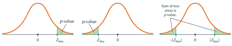
Note that the -value has precisely the same definition and behavior as in the test for the population mean . That is, the -value is roughly a measure of how extreme your value of is and takes values between 0 and 1, with small values indicating extreme values of .
Developing Your Statistical Sense
The Difference Between the -Value and the Population Proportion
Be careful to distinguish between the -value and the population proportion p. The latter represents the population proportion of successes for a binomial experiment and is a population parameter. The -value is the probability of observing a value of at least as extreme as the actually observed. The -value depends on the sample data, but the population proportion does not depend on the sample data.
test for the Population Proportion : -value Method
When a random sample of size is taken from a population, you can use the test for the proportion if both of the normality conditions are satisfied:
547
Step 1 State the hypotheses and the rejection rule.
Use one of the forms from Table 12. State the meaning of . State the rejection rule as “Reject when the .”
Step 2 Calculate .
Step 3 Find the -value.
Either use technology to find the -value, or calculate it using the form in Table 12 that corresponds to your hypotheses.
Step 4 State the conclusion and the interpretation.
If the , then reject . Otherwise, do not reject . Interpret your conclusion so that a nonspecialist can understand.
EXAMPLE 27 test for using the -value method

We report to two decimal places to allow the use of the table to calculate the -value.
The National Transportation Safety Board publishes statistics on the number of automobile crashes that people in various age groups have. Young people ages 18–24 have an accident rate of 12%, meaning that on average 12 out of every 100 young drivers per year had an accident. A researcher claims that the population proportion of young drivers having accidents is greater than 12%. Her study examined 1000 young drivers ages 18–24 and found that 134 had an accident this year. Perform the appropriate hypothesis test using the -value method with level of significance .
Solution
First, we check that both of our normality conditions are met. We are interested in whether the proportion has increased from 12%, so we have .
The normality conditions are met and we may proceed with the hypothesis test.
Step 1 State the hypotheses and the rejection rule.
Our hypotheses are
where represents the population proportion of young people ages 18–24 who had an accident. We reject the null hypothesis if the .
Step 2 Calculate .
Our sample proportion is . Because , the standard error of is
Thus, our test statistic is
548
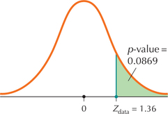 Figure 9.46: FIGURE 36 -Value for a right-tailed test equals area to right of .
That is, the sample proportion lies approximately 1.36 standard errors above the hypothesized proportion .
Step 3 Find the -value.
We have a right-tailed test, so our -value from Table 12 is . This is a Case 2 problem from Table 8 in Chapter 6 (page 355), where we find the tail area by subtracting the table area from 1 (Figure 36):
Step 4 State the conclusion and the interpretation.
The -value 0.0869 is not ≤ , so we do not reject . There is insufficient evidence that the population proportion of young people ages 18–24 who had an accident has increased.
NOW YOU CAN DO
Exercises 19–22.
YOUR TURN #12
For Example 27, suppose 150 of the 1000 young drivers ages 18–24 had an accident this year. Now test whether the population proportion of young drivers who had an accident exceeds 0.12, using level of significance, .
(The solution is shown in Appendix A.)
EXAMPLE 28 Performing the test for using technology
A study reported that 1% of American Internet users who are married or in a long-term relationship met on a blind date or through a dating service.13 A survey of 500 American Internet users who are married or in a long-term relationship found 8 who met on a blind date or through a dating service. If appropriate, test whether the population proportion has increased. Use the -value method with level of significance .
Solution
We have and . Checking the normality conditions, we have
The normality conditions are met and we may proceed with the hypothesis test.
Step 1 State the hypotheses and the rejection rule.
Our hypotheses are
where represents the population proportion of American Internet users who are married or in a long-term relationship and who met on a blind date or through a dating service. We will reject if the -value # 0.05.
Step 2 Calculate .
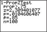
We use the instructions supplied in the Step-by-Step Technology Guide on page 552. Figure 37 shows the TI-83/84 results from the test for , Figure 38 shows the results from Minitab, and Figure 39 shows the results from CrunchIt!.
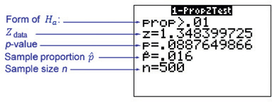 Figure 9.47: FIGURE 37 TI-83/84 results.
549
Note: Minitab, TI-83/84, and CrunchIt! round results to different numbers of decimal places.
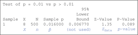 Figure 9.48: FIGURE 38 Minitab results.
We have
which concurs with the TI-83/84 results in Figure 37.
Step 3 Find the -value.
From Figures 37, 38, 39, and 40 we have
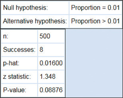 Figure 9.49: FIGURE 39 CrunchIt! results.
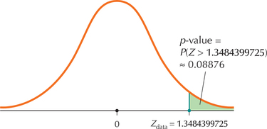 Figure 9.50: FIGURE 40 -Value for a right-tailed test.
Step 4 State the conclusion and interpretation.
Because is , we do not reject . There is insufficient evidence that the population proportion of American Internet users who are married or in a long-term relationship and who met on a blind date or through a dating service has increased.
3 Using Confidence Intervals for to Perform Two-Tailed Hypothesis Tests About
Just as for , we can use a confidence interval for the population proportion in order to perform a set of two-tailed hypothesis tests for .
EXAMPLE 29 Using a confidence interval for to perform two-tailed hypothesis tests about
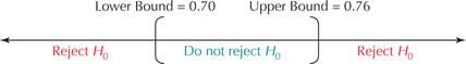
In 2013, Facebook reported that 73% of its users access Facebook using a mobile device. Suppose that a 95% confidence interval for the population of mobile accessers is (lower bound = 0.70, upper bound = 0.76). Use the confidence interval to test, using level of significance , whether the population proportion differs from
550
- 0.69
- 0.72
- 0.77
Solution
There is equivalence between a confidence interval for and a two-tailed test for with level of significance . Values of that lie outside the confidence interval lead to rejection of the null hypothesis, whereas values of within the confidence interval lead to not rejecting the null hypothesis. Figure 41 illustrates the 95% confidence interval for .
We want to perform the following two-tailed hypothesis tests:
To perform each hypothesis test, simply observe where each value of falls on the number line. For example, in the first hypothesis test, the hypothesized value lies outside the interval (0.70, 0.76). Thus, we reject . The three hypothesis summarized here.
| Value of | Form of hypothesis test, with |
Where lies in relation to 95% confidence interval |
Conclusion of hypothesis test |
|---|---|---|---|
| a. 0.69 | Outside | Reject | |
| b. 0.72 | Inside | Do not reject | |
| c. 0.77 | Outside | Reject |
NOW YOU CAN DO
Exercises 23–26.
EXAMPLE 30 interpreting software output
Each of (a) and (b) represent software output from a test for . For each, examine the indicated software output, and provide the following steps:
- Step 1 State the hypotheses and the rejection rule.
- Step 2 Find .
- Step 3 Find the -value.
- Step 4 State the conclusion and the interpretation.
Use level of significance for each hypothesis test.
- TI-83/84 output for a test for p, where represents the population proportion of quiz questions answered correctly.
551
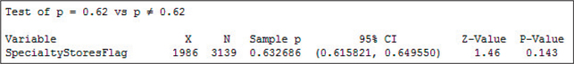
- Minitab output for a test for , where represents the population proportion of counties having at least one specialty store.
Solution
- Interpreting the TI-83/84 output
Step 1 State the hypotheses and the rejection rule.
In the TI-83/84 output, the “” tells us that we have a right-tailed test:
where represents the population proportion of quiz questions answered correctly. We will reject if the -value is less than the level of significance
Step 2 Find .
The “” in the TI-83/84 output gives us the value for .
Step 3 Find the -value.
Here, we need to be a little bit careful, because there are two items containing in the TI-83/84 output. Don't pick , which represents the sample proportion of successes. Instead, the -value is given as “.”
Step 4 State the conclusion and the interpretation.
The -value is less than the level of significance , so we reject . There is evidence that the population proportions of quiz questions answered correctly is greater than 0.75.
Interpreting the Minitab output
Step 1 State the hypotheses and the rejection rule.
The line “Test of vs ” tells us that we have the following two-tailed test.
where represents the population proportion of counties having at least one specialty store. We will reject if the -value is less than the level of significance .
Step 2 Find .
The “-value” of 1.46 in the Minitab output gives us the value for .
Step 3 Find the -value.
Under “P-Value,” Minitab gives us .
Step 4 State the conclusion and the interpretation.
The -value is not less than the level of significance , so we do not reject . There is insufficient evidence that the population proportions of counties having at least one specialty store differs from 0.62.
NOW YOU CAN DO
Exercises 27–30.
552