12.3 12.2 Spatial Models for Two-Candidate Elections: Discrete Distributions
Two-candidate contests are most common in the general election—but occasionally there are other significant candidates. One example is Ross Perot, who ran under the banner of the Reform Party in 1992 and garnered 19% of the popular vote. Although no minor-party candidate has ever won a presidential election, some have affected which of the two major-party nominees did win. For example, Ralph Nader impacted the 2000 presidential election, in part because many voters who voted for Nader in Florida would have voted for Al Gore otherwise and, consequently, would have tipped the election in Gore’s favor. We begin with the situation in which there are just two candidates in the general election.
To model such elections, we assume that voters respond to the candidates’ positions on various issues. This is not to say that other factors—such as personality, ethnicity, religion, and race—have no effect on election outcomes, but rather that issues take precedence in a voter’s decision. How can a candidate’s position be represented? We start by assuming that there is a single overriding issue, or set of issues, on which the candidates must take a definite stand, such as the degree of governmental intervention in the economy. We assume that the voters’ attitudes on this issue or dimension can be represented along a left-right continuum, ranging from very liberal on the left (much intervention) to very conservative on the right (little intervention).
Other examples of one-dimensional issues include the amount of military buildup, the amount of foreign aid to developing countries, and so on. Geometrically, the left-right continuum is a portion of the real line. For example, foreign aid can be represented in dollars and can range from “no foreign aid” (i.e., 0 on the number line) to any positive dollar amount.
To derive conclusions about the behavior of voters from their attitudes and the positions candidates take in a campaign, some assumption is necessary about how voters decide for whom to vote. We assume that a candidate announces a policy position—a point on the left-right spectrum. Voters are assumed to vote for the candidate whose policy position is closest to the voter’s ideal position, often called the voter’s ideal point—the favorite position of the voter. For two candidates and with distinct policy positions , a voter with ideal point votes for Candidate if and votes for Candidate if . The voter’s ideal point is equidistant from and if . In this case, the voter is indifferent to the choice between the two candidates and could choose to vote for either one, possibly based on some other criterion used as a tiebreaker. The position is key and is related to geometry.
509
Algebra Review Appendix
Distance and Midpoint Between Two Points on a Line
Midpoint DEFINITION
For points and on the real line, the midpoint is . Because and are numbers, is also called the arithmetic average, or average.
For a two-candidate election, which candidate a voter votes for depends on how the voter’s ideal point compares to the midpoint of the candidates’ policy positions. To determine which candidate wins the election, each voter’s ideal position is compared with the midpoint. For this reason, the number of voters who have particular attitudes along the left-right continuum is often more important than the attitude of any individual voter. A distribution of voters describes or counts the numbers of voters with each ideal point.
Discrete Distribution of Voters DEFINITION
A discrete distribution of voters counts the number of voters whose ideal points are located at any point along the left-right continuum.
EXAMPLE 3 Determining the Winner of an Election in a Spatial Model
Suppose that there are 21 eligible voters in a tiny town who must decide between Ann and Bob for mayor. Each voter has an ideal position that describes how much of the town’s taxes should be used to subsidize child care. A voter with an ideal position closer to 0 desires a higher subsidy. As the voter’s ideal point increases, then the voter prefers a smaller subsidy. The 21 voters have 7 distinct ideal positions, as described by the discrete distribution given in Table 12.5. For example, there are 4 voters who have 6 as their ideal position.
| Ideal points | 0 | 2 | 3 | 4 | 6 | 8 | 10 |
| Number of voters | 1 | 3 | 6 | 3 | 4 | 2 | 2 |
As part of their election platforms, Ann and Bob announce their positions on the child-care subsidy. Bob is more supportive of the child-care subsidy, having announced a position of 2 on the 0 to 10 scale. Ann is less supportive, having announced a position of 7. Each voter votes for the candidate whose announced position is closest to his or her ideal position. Figure 12.1 shows a graphical representation of the voters’ ideal points, as well as the policy positions announced by Ann (red line) and Bob (blue line).
510
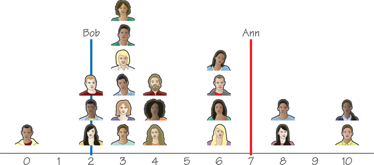
Voters at positions 0, 2, 3, and 4 all vote for Bob because each of these positions is to the left of the midpoint and therefore closer to Bob’s position of 2 (the blue line in Figure 12.1) than Ann’s position of 7 (the red line in Figure 12.1). For example, the distance between a voter’s ideal position 4 and Bob’s position 2 is , whereas the distance to Ann’s position is . Because 2 is less than 3, a voter with ideal position 4 votes for Bob over Ann. The other voters with ideal positions at 6, 8, and 10 vote for Ann over Bob because their ideal positions are greater than the midpoint and are closer to Ann’s position of 7 than Bob’s position of 2. Consequently, 13 of the 21 voters vote for Bob and 8 of the 21 voters vote for Ann. Bob wins the election.
What if Ann now thinks about how she could have changed her policy position? If she had announced a position to the right of Bob’s 2, then the best she could have hoped for is that all voters with ideal positions greater than 2 voted for her. There are 17 such voters. If Ann wanted to attract these 17 voters and win the election, then she could have announced a policy position of 3 or any other policy position greater than 2 and less than 4. However, if she had announced a policy position of 4, she would have still won the election, receiving 11 of the 21 votes. In fact, the policy position 4 has a special property: it is the median of the distribution.
Self Check 3
If Ann had announced a policy position of 5 instead of 7, then which voters would have voted for Ann and which for Bob? Who would have won the election?
- If Ann announced a policy position of 5 instead of 7, then the midpoint between Bob’s position of 2 and Ann’s position of 5 is . All voters with ideal points less than 3.5 vote for Bob. There are 10 such voters. The 11 other voters with ideal points greater than 3.5 vote for Ann. Ann wins the election.
Self Check 4
Suppose that Ann announces policy position 4 and Bob announces policy position 3.9. Who wins the election? What if Bob announces policy position 4.1? Who wins the election?
- If Ann announces the policy position 4 and Bob announces 3.9, then voters with ideal points greater than or equal to 4 vote for Ann. There are 11 such voters, so Ann wins the election 11 to 10. If Bob changes his policy to 4.1, then the 11 voters with ideal points less than or equal to 4 now vote for Ann. Ann still wins the election 11 to 10.
511
Median DEFINITION
The median of a distribution of voters’ ideal points is a point on the horizontal axis where at least half the voters have ideal points that are equal or to the left of the point and where at least half the voters have ideal points that are equal or to the right of the point.
In practice, with an odd number of voters, finding the median requires listing all the ideal points and counting. For the distribution in Example 3, the following list contains all voters’ ideal points from least to greatest:
In the list, each ideal point appears as many times in the list as there are voters that share the ideal point. There are 21 numbers in the list, and the bolded 4 is the eleventh, or middle, entry in the list—this is the median of the distribution, so .
In Self Check 4, you determined that Ann would’ve won the election if Bob had announced a policy position of 3.9 or 4.1. In fact, Bob cannot defeat Ann with any policy position less than 4 because 11 of the voters have ideal points greater than or equal to 4. However, Bob cannot defeat Ann with any policy position greater than 4 because 11 of the voters have ideal points less than or equal to 4. Ann’s policy position is undefeatable! The observation that 4 is an undefeatable position is generalized through the following definitions.
Maximin DEFINITION
A position is maximin for a candidate if there is no other position that can guarantee a better outcome—more votes for that candidate—whatever position the other candidate adopts.
In an election in which two candidates choose distinct policy positions and there is an odd number of voters, a candidate is guaranteed more than 50% of the total vote by selecting a position at , regardless of what the other candidate does. Moreover, there is no other position that can guarantee the candidate with the median position more votes—and likewise for the opponent. If both candidates choose , voters will be indifferent to their choices between the candidates on the basis of the announced policy positions alone and would presumably make their choices on other grounds. is also stable, because if one candidate adopts this position, the other candidate has no incentive to choose any position other than .
If Ann were to change her policy position in Example 3, then she should change it to . Thus, is both the maximin position for each candidate (it offers a guarantee of a minimum of 50% of the votes), and if both candidates choose , then these choices are in equilibrium (one candidate does worse by departing from if the other candidate stays at ).
Equilibrium DEFINITION
A pair of positions is in equilibrium if, once chosen by both candidates, neither candidate has an incentive to depart from it unilaterally (i.e., by himself or herself).
512
More formally, we have the median-voter theorem.
Median-Voter Theorem THEOREM
In a two-candidate election with an odd number of voters, is the unique equilibrium position. (The theorem is applicable if there is an even number of voters, as we show later.)
We required an odd number of voters for convenience. The same type of analysis is possible for an even number of voters. The difficulty is that if there were an even number of voters, then there may be more than one policy position that satisfies the definition of a median, as demonstrated in the following example.
EXAMPLE 4 A Discrete Distribution with an Even Number of Voters
Suppose that a Home Owner Association of a condominium complex wants to build a swimming pool and clubhouse for its residents along a 1-mile stretch of road. Residents live in one of six buildings, and each building gets a single vote to indicate its ideal point for where the clubhouse and pool should be located. Let the line segment from 0 to 1 represent the 1-mile stretch of road on which to build the facility. Suppose the six buildings have ideal points, ordered from smallest to largest, of 0.1, 0.3, 0.3, 0.5, 0.8, and 0.9. A Building Company (ABC) and Barry’s Builders are to propose different locations on the road—policy positions—for the new facility. Where should they build it?

Because there are 6 locations, there is no middle item in the list: 0.1, 0.3, 0.3, 0.5, 0.8, 0.9. That is, there is no median value in the list. In the absence of such a median position, is there still an equilibrium? It is not too difficult to show that if a discrete distribution has an even number of voters, then there is at least one equilibrium position. In fact, there may be a range of policy positions that, when paired, are in equilibrium with one another.
Suppose that ABC proposes to build at 0.4 and Barry proposes to build at 0.5. Each builder will receive half of the votes: Buildings with ideal points 0.1 and 0.3 vote for ABC, while the other buildings vote for Barry. If Barry were to change the proposed building site, notice that he could do no better than receiving 3 of the 6 votes. Indeed, this is the case for ABC, too.
This example can be generalized as follows: If ABC and Barry each announce distinct positions between 0.3 and 0.5, inclusive, then each builder will receive half the votes. This is no accident, as 0.3 and 0.5 are the two middle values in the ordered list of ideal points. Furthermore, if each builder announces a position between 0.3 and 0.5, inclusive, then neither builder will have an incentive to change. They will be in equilibrium. For this example, we call the interval [0.3, 0.5] of policy positions the extended median of the discrete distribution.
Extended Median DEFINITION
For a discrete distribution of an even number (say, ) of voters’ policy positions, the extended median is the set of positions between, and including, the th and st values of the list of the voters’ ideal points, ordered from least to greatest.
513
In statistics, when there are items in an ordered list, the average of the th and st is usually defined as the median. For a discrete distribution of an even number of ideal points, if the th and st values are the same, then there is still just a single median; otherwise, no single value satisfies the definition of median. The policy positions that define the extended median are so-called because they extend the median-voter theorem to an even number of voters.
Self Check 5
Find the range of values that make up the extended median if the voters’ ideal points are 0, 1, 1, 2, 2, 3, 3, 3, 3, and 4.
- There are 10 numbers in the list 0, 1, 1, 2, 2, 3, 3, 3, 3, 4. The 5th and 6th numbers in the list are 2 and 3. The extended mean is the interval [2, 3].
The spatial models considered so far can be modified to model situations in which voters prefer candidates with policy positions farther from their ideal points and to consider elections in which there is more than one important issue. Such situations are demonstrated in the next two examples.
EXAMPLE 5 Wind Farm Location: NIMBY (Not In My backyard)
Up to this point, we assumed that a voter would vote for a candidate whose policy position was closest to the voter’s ideal position. In the following example, assume that the election is to determine the location of a wind farm off a coastline—a left-right continuum. Although many voters appreciate that a wind farm generates clean energy, voters do not want to have the wind farm ruin their views. That is, numerous voters may prefer a wind farm but don’t want it to be built “in their backyard.”

There may be other reasons not to support a wind farm. Indeed, a plan to install a wind farm of 170 wind turbines off the coast of Cape Cod, Massachusetts, split normally similarly spirited organizations into camps for and against the proposal. For example, the Humane Society, International Fund for Animal Welfare, and environmental lawyer Robert F. Kennedy, Jr., were against the placement of a wind farm off of Cape Cod because the wind turbines can be harmful to animals. However, the Natural Resources Defense Council, the Union of Concerned Scientists, and Greenpeace supported the wind farm.
Suppose that the 15 voters who live along the coast of a small island determine the placement of a wind farm. Like the child-care funding example (Example 3 on page 509), the voters have positions on a left-right continuum from 0 to 100. A voter’s ideal point could represent his or her house and the preference that the wind farm be as far away as possible so that it does not ruin the ocean view. Hence, for this example, voters vote for the location that is farthest away from their ideal points.
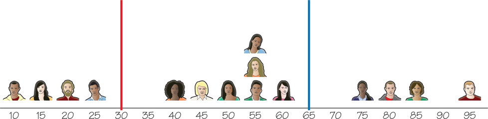
Let the 15 voters live at the following positions: 10, 15, 20, 25, 40, 45, 50, 55, 55, 55, 60, 75, 80, 85, and 95, as depicted in Figure 12.2. Assume that there are two proposals for the location of the wind farm: one at 30 and the other at 65. Voters with residences closer to position 30 vote for the wind farm to be built at 65. Similarly, voters with residences closer to position 65 vote for the wind farm to be built at 30. Even though voters now prefer the location or policy position that is farthest from their ideal points, the midpoint still plays a central role. The midpoint between 30 and 65 is . Voters who reside at locations less than 47.5 are closer to location 30. These 6 voters vote for the wind farm to be built at location 65. The other 9 voters reside at locations greater than 47.5 and are closer to 65. They vote for the wind farm to be built at location 30. Because more voters are closer to location 65 than to location 30, the wind farm will be built at location 30.
514
Although some elections have a single dominant issue (such as when campaign strategist James Carville’s “The economy, stupid” became a rallying cry in Bill Clinton’s 1992 presidential campaign against incumbent George H. W. Bush), other elections may have more than one salient issue. Spatial models are still relevant. And the midpoint still plays an important role.
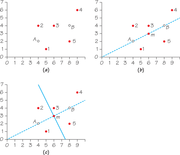
EXAMPLE 6 Two-Dimensional Spatial Voting
Five board members of a company must decide between two other board members ( and ) for the vaunted position of chairman of the board. The voters are concerned with two issues: overseas expansion and the timing of the initial public offering. The voters’ ideal points and the candidates’ policy positions are ordered pairs , where indicates the position on overseas expansion (a larger value of means a more vast expansion) and where indicates the time until the initial public offering (a larger value of represents a longer time until the initial public offering will be held).

Algebra Review Appendix
Plotting Points in the Plane
Assume that and announce policy positions of (4, 2) and (8, 4), respectively. The ideal points of board members 1 through 5 are (5, 1), (4, 4), (6, 4), (9, 6), and (8, 2), respectively. The policy and ideal positions are graphed in Figure 12.3a.
Algebra Review Appendix
Distance and Midpoint Between Two Points in the Plane
The midpoint of (4, 2) and (8, 4) is on the line that connects these points; this is the dashed line in Figure 12.3b. The midpoint is calculated by taking the average of each coordinate. The -coordinate of the midpoint is and the -coordinate of the midpoint is . Equivalently, the midpoint satisfies
Just as the midpoint of two policy positions divides the left-right continuum into three regions in which (1) voters prefer one policy position, (2) voters prefer the other policy position, and (3) voters are indifferent to the choice between the two policy positions, there is also a way to use the midpoint to divide the two-dimensional policy space into three similar regions. In high school geometry, we learn how to draw a line through a point that is perpendicular to another line, using either a compass or dynamic geometry software.
The solid line in Figure 12.3c is through the midpoint and is perpendicular to the dashed line between the policy positions of and . It divides the two-dimensional space so that voters with ideal points below the solid line prefer over , voters with ideal points above the solid line prefer over , and voters with ideal points on the solid line are indifferent between and . Board members 3, 4, and 5 have ideal points above the solid line and vote for Candidate , while board members 1 and 2 have ideal points below the solid line and vote for Candidate . Board member is elected as chairman of the board.
515