4.4 4.3 Why the Corner Point Principle Works
In finding solutions to our mixture problems, we have been using the corner point principle, which says that the highest profit value on a convex polygonal feasible region is always at a corner point. A feasible region has infinitely many points, making it impossible to compute the profit for each point. The corner point principle gives us a finite set of points, making the calculation possible.
You can visualize a mathematical proof of the corner point principle by imagining that each point of the plane is a tiny light bulb that is capable of lighting up. For the juice mixture example, whose feasible region is shown in Figure 4.9c, imagine what would happen if we ask this question: Will all points with profit = 360 please light up? What geometric figure do these lit-up points form?
In algebraic terms, we can restate the profit question in this way: Will all points () with please light up? As it happens, this version of the profit question is one that mathematicians learned to answer hundreds of years before linear programming was born.
The points that light up make a straight line because is the equation of a straight line. Furthermore, it is a routine matter to determine the exact position of the line. We call this line the profit line for 360; it is shown in Figure 4.10. For numbers other than 360, we would get different profit lines. Unfortunately, there are no points on the profit line for 360 that are feasible—that is, which lie in the feasible region. Therefore, the profit of 360 is impossible. If the profit line corresponding to a certain profit value doesn’t touch the feasible region, then that profit value isn’t possible.
Because 360 is too big, perhaps we should ask the profit line for a more modest amount, say, 160, to light up. You can see that the new profit line of 160 in Figure 4.10 is parallel to the first profit line and closer to the origin. This is no accident: All profit lines for the profit formula have the same coefficients for and —namely, 3 for and 4 for . Because the slope of the line is determined by those coefficients, they all have the same slope. Changing the profit value from 360 to 160 has the effect of changing where the line intersects the y-axis, but it does not affect the slope. These different profit lines are parallel to each other.
142
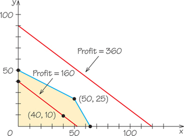
The most important feature of the profit line for 160 is that it has points in common with the interior of the feasible region. For example, (40, 10) is on that profit line because ; in addition, (40, 10) is a feasible point. This means that it is possible to make 40 gallons of cranapple and 10 gallons of appleberry and that if we do so, we will have a profit of 160.
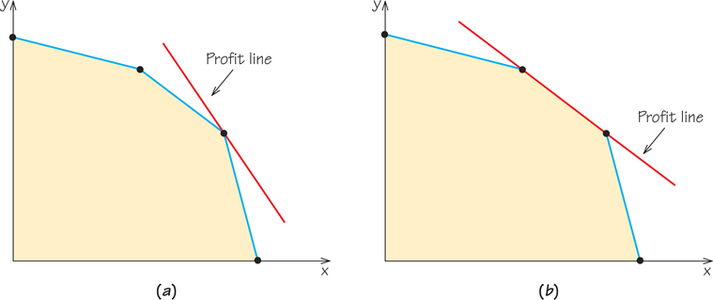
Can we do better than a 160 profit? As we slowly increase our desired profit from 160 toward 360, the location of the profit line that lights up shifts smoothly upward away from the origin. So long as the line continues to cross the feasible region, we are happy to see it move away from the origin because the more it moves, the higher the profit represented by the line. We would like to stop the movement of the line at the last possible instant, while the line still has one or more points in common with the feasible region. It should be obvious that this will occur when the line is just touching the feasible region either at a corner point (Figure 4.11a) or along a line segment joining two corners (Figure 4.11b). That point or line segment corresponds to the production policy or policies with the maximum achievable profit. This is just what the corner point principle says: The maximum profit always occurs at a corner or along an edge of the feasible region.
143
EXAMPLE 7Adding Nonzero Minimums: beverages
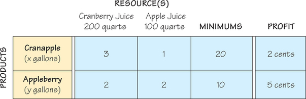
Suppose that in Example 6, the profit for cranapple changes from 3 cents per gallon to 2 cents and the profit for appleberry changes from 4 cents per gallon to 5 cents. You can verify that this change moves the optimal production policy to the point (0, 50); no cranapple is produced. This result is not surprising: Appleberry is giving a higher profit and the policy is to produce as much of it as possible. But suppose the manufacturer wants to incorporate nonzero minimums into the linear-programming specifications so that there will always be both cranapple, , and appleberry, , produced. Specifically, the manufacturer decides that and are desirable minimums. Figure 4.12 is the mixture chart showing the new profit formula and the nonzero minimums, along with the unchanged rest of the beverage problem.
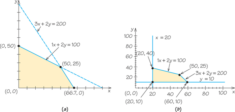
The feasible region for beverages in Example 6 is shown in Figure 4.13a. The feasible region for beverages in this example is shown in Figure 4.13b. You can verify that, starting at the lower-left corner of the new feasible region and moving clockwise around its boundary, we have corner points (20, 10), (20, 40), (50, 25), and (60, 10). (One of those points was also a corner point of the old feasible region. Can you explain why?) Table 4.6 shows the evaluation of the profit formula at these corner points. For this modified problem, the optimal production policy is to produce 20 gallons of cranapple and 40 of appleberry, for a maximum profit of 240 cents.
144
| Corner Point | Value of the Profit Formula: |
|---|---|
| (20, 10) | |
| (20, 40) | |
| (50, 25) | |
| (60, 10) |
One final note about this solution concerns the resources. The point (20, 40) is on the resource constraint line for the apple juice resource, so it represents using up all the available apple juice. We can see this by inserting the apple juice resource constraint: is true. However, (20, 40) is below the line for the cranberry juice resource, indicating that there will be slack, or leftover, amounts of cranberry juice. Specifically, substituting (20, 40) into the cranberry juice constraint gives , which is 60 quarts less than the 200 quarts available. The slack is 60 quarts of cranberry juice. Dealing with slack can be an important consideration for manufacturers. Can you see why?