4.6 4.5 A Transportation Problem: Delivering Perishables
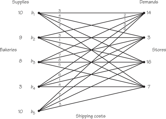
A supermarket chain gets bread deliveries from a bakery chain that does its baking in different places. Each supermarket store needs a certain number of loaves each day, and the supplier bakes, in total, enough breads to exactly meet the demands. Figure 4.17 shows the cost to ship a loaf from a particular baking location to the store involved. How many breads should be shipped from each locale to each of the stores to stay within the demands and to minimize the cost?
Similarly, after a long holiday weekend, a car rental company will have extra cars in some cities and too few cars in other cities. It is faced with the problem of reshuffling the cars at minimal cost so that each city has the right number of cars. Companies that provide bicycles for use at specific hire/drop locations in urban areas face similar issues. Problems such as these go under the general name of transportation problems, and they form a special class of linear-programming problems that can be solved by a specialized method.
149
Transportation Problem DEFINITION
A group of suppliers must meet the needs of users of these supplies. There is a cost for shipping from a particular supplier to a particular user (demander). The transportation problem involves minimizing the total shipping cost of meeting the required demands from the supplies available.
EXAMPLE 8 Delivering Bread
Imagine that we have three bakeries and three stores, though the ideas we develop will also solve problems where the number of stores and bakeries are not the same. The three stores require 3 dozen, 7 dozen, and 1 dozen loaves of bread, respectively, while the three bakeries can supply 8 dozen, 1 dozen, and 2 dozen loaves, respectively. The information given so far can be displayed in Figure 4.18, where the “suppliers” are represented by the rows of the table (labeled with Roman numerals) and the “demanders” are represented by the columns (labeled with Hindu-Arabic numerals).
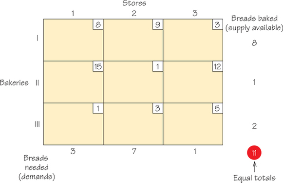
The numbers of breads available and the numbers being required are shown on the right side and bottom of the table and will be referred to as rim conditions. Each entry of the table shown in Figure 4.18 is known as a cell. it is convenient to have a name for each of these cells. For example, the cell in the third row and second column will be denoted (III, 2). The first number always corresponds to a row, the second to a column. Thus cell (I, 2) refers to Bakery I and Store 2.
In deciding which bakeries should ship to which stores, it seems natural to take into account the costs of shipping a dozen breads from a particular bakery to a particular store. if Bakery I is farther from Store 2 than is Bakery II, it seems reasonable that the shipping cost for I will be higher than for II when shipping to that particular store.
150
However, the costs of shipping may also involve time considerations. (The distance to a store may be shorter, but it may be that this route is a very slow one.) Also, it may take extra time for a truck coming from I to park when making the next delivery.
The numbers we use in our diagrams are “aggregate” costs. The nice thing about what we are doing is that the solution method works independently of the way the costs are arrived at or computed. These costs (see Figure 4.18) are shown in the upper- right-hand corner of a cell. Thus the number 9 shown in cell (I, 2) means that it costs nine units to ship a bread from Bakery I to Store 2. Our goal will be to supply the stores with the breads they require from the supplies available at the bakeries so that the total cost of providing the breads to the stores is as small as possible (a minimum).
The tools for solving transportation problems like these were developed during World War II in conjunction with getting supplies from different ports in the United States to different ports in Europe (mostly the United Kingdom) as efficiently as possible. (The U.S. ports were like the bakeries, and the British ports were like the stores that needed the breads.)
We can think of finding a solution to a problem like this as a special kind of linear-programming problem because we can express the objective of minimizing the cost using a linear relationship. The constraints that express that the rim conditions are met can also be expressed using linear equations. However, it turns out there are algorithms that make it possible to solve problems of this kind that are rather larger than general linear-programming problems which can be solved by hand. These algorithms are intuitively appealing.
We can divide the problem of finding a solution to a transportation problem into two phases, as we did for general linear-programming problems. First, find a solution that is feasible (that is, a solution that does not violate any of the constraints of the problem). Second, if the current solution is not optimal, we move to a better one. Thus, we will first find a solution that meets the constraints and then try to find an improved solution. If there is no better solution than the one we have, under suitable circumstances we show that there is never a better one. Thus, the solution that we have found is an optimal solution. We will work our way through a simple example that is typical of what is required in general transportation problems.
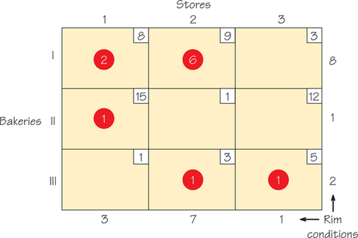
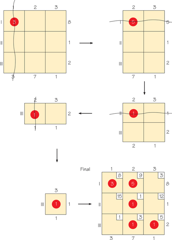
Let’s turn to the table shown in Figure 4.19, where certain numbers have been inserted with circles around them.
151
Tableau DEFINITION
A table showing costs and rim conditions for a transportation problem is known as a tableau.
When we see a circled number such as the 6 in row I, column 2, this means that we plan to ship six breads to Store 2 from Bakery I. Similarly, the circled number 1 in row III and column 3 means we plan to ship one bread from Bakery III to Store 3. The cells that have no circled numbers are thought of as having zero entries; no breads are being shipped between these stores and these bakeries. Note, for example, that the row sum of the circled numbers in the first row is 8. This means that all the breads available at Bakery I are being shipped to some store.
Similarly, the fact that the circled entries in column 2 add up to 7 means that all the breads needed by Store 2 are being supplied to it. You can verify that all the row sums and column sums add to exactly the numbers that we want to ship from each bakery to each store. Note that 11 breads have been shipped by the bakeries and received by the stores. When this happens, the circled numbers are said to be a feasible solution to the problem.
How much will it cost to ship these amounts of breads (see Figure 4.19) to the stores? The number can be computed by multiplying the circled numbers by the cost shown in the associated cell. For example, to ship two breads from Bakery I to Store 1 costs because the cost associated with the cell in which the 2 appears is 8. The cost of shipping six breads from Bakery I to Store 2 is . To get the total cost of this “shipment plan,” we sum all the shipped amounts by the associated costs to get
However, at this point we do not know if there is a cheaper way to ship the breads to the stores. Notice that the number of cells with circled numbers is exactly equal to the number of rows plus the number of columns . This is the general pattern with transportation problems. Cells that are used for shipping are circled. On occasion, we ship a zero amount because the procedure works only when cells are circled.
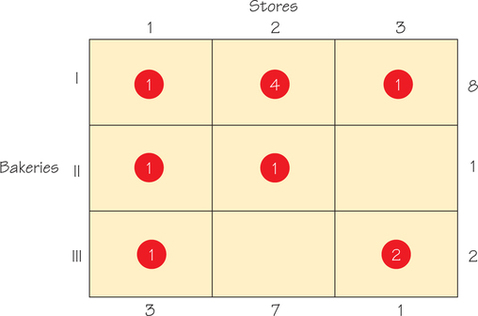
If we look at the pattern of circled numbers in the tableau in Figure 4.20, we see that there is a difficulty even though 11 breads are involved (the sum of all the circled numbers).
152
The numbers in the first row add to 6, which means that at Bakery I there will be breads left over that have not been shipped. In row 2, the sum of the circled numbers is 2, but this means that something is wrong. How can Bakery II, which has a supply of only 1 bread, ship 2 breads? Furthermore, column 3 sums to 3, which means that 3 breads have been shipped to Store 3 despite the fact that it only requested 1 bread! These facts add up to the realization that this assignment of numbers to the cells violates the rules we are requiring. This proposed shipment plan also violates our rule that we are not allowed to circle more than five cells.
How can we find a solution that meets the constraints of the problem (the rim conditions)? We will show two ways to do this. The first is “fast and dirty” but typically does not find a very good solution with which to start. The second (developed in the exercises) usually gives a better “initial” solution but is a little harder to carry out.
This pair of approaches displays a common tension in problem solving: the ease of getting started but requiring more work later on, or more work at the start, which often proves to be a good investment of extra effort because less work is needed to find an optimal solution. If we know in advance the method being chosen to solve a problem, we can often find an example where this particular method does poorly. Mathematicians work hard to find methods that work well on the kinds of problems that come up in genuine applications.
Northwest Corner Rule
The easier approach involves what is called the Northwest Corner Rule. This rule is simple because it is based on the geometry of the table that is involved and does not even look at the costs associated with the cells in the table, which in the long run cannot be a good idea, because these costs come into play when trying to get an optimal solution.
How does the Northwest Corner Rule work? The algorithm carries out the following procedure until exactly one cell remains in the “altered tableau.”
Northwest Corner Rule PROCEDURE
- Locate that cell of the current tableau that is as far to the top and to the left as possible (that is, in the northwest corner). Ship via this cell the smaller of the two rim values (call the value ) associated with the row and column of this cell. (Indicate that this cell is being used by putting a circle around the entry in the tableau.)
- Cross out the row or column that had rim value and reduce the other rim value for this cell by .
- When a single cell remains, there will be a tie for the rim conditions of both the row and column involved, and this amount is entered into the cell and circled.
Note that it is possible (when there is more than one cell at the start) for there to be a tie when Step 1 above is applied. In this case, we simultaneously fulfill the rim conditions for a row and column. If this happens, we can always choose to cross out, say, the column (not both the row and column) and reduce to 0 the rim condition for the row involved. Now when the algorithm is applied, one has a rim value of 0 for the northwest corner cell. This now requires that 0 be shipped via that cell. Even though this will not change the cost, it is necessary to put a 0 in this cell and circle it. Here we have usually designed the examples to avoid ties so as to make it easier to get the essential ideas across.
153
EXAMPLE 9 Using the Northwest Corner Rule
Applying the Northwest Corner Rule to our original tableau (see Figure 4.18), we get the sequence of tableaux in Figure 4.21 as we cross out the rows or columns, where for clarity the costs associated with the cells are suppressed. The last diagram in the sequence shows the results on the original tableau, with the cost restored. Note that, at the steps in between, the costs played no role. it is a good idea to check that the circled numbers in each row and column really add up to the rim value for that row and column and that exactly cells are filled.
We can now compute the cost of the associated solution that we have found (feasible solution), which obeys the rim conditions. As we did previously, we add up the cost multiplied by the amount shipped for each cell with a circled entry. We get the following calculation:
154
This shows a cost that is smaller than the solution we found earlier. That solution involved a cost of 93. But is this solution the cheapest one? The fact that this feasible solution was found without using the costs on the cells suggests that no, it is not very likely this solution is cheapest.
Improving the Feasible Solution
The next phase of the transportation problem algorithm attempts to answer the question of how to tell if the feasible solution found by using the Northwest Corner Rule is the best. If this solution is not the best, we should be able to find a way to improve it.
Suppose that we decided to ship an additional bread from Bakery II to Store 3. Now, this would violate the fact that we had shipped exactly the right numbers of breads before this new additional shipment, so we have shipped 1 bread too many from Bakery II. We can compensate for this by reducing from 1 to 0 the bread shipped from Bakery II to Store 2. But this now means that Store 2 has not gotten all the breads it needs. We can take care of this by shipping 1 more bread from Bakery III to Store 2, but again we now have 1 extra bread shipped from Bakery III. We can compensate for this by reducing the number of breads shipped via cell (III, 3)—that is, from Bakery III to Store 3. This step will ensure that the rim conditions will hold for the circled numbers. This is because we have located a circuit—(II, 3), (II, 2), (III, 2), (III, 3), (II, 3)—where, if we increase and decrease the breads alternately going around that circuit, we maintain the rim conditions (see Figure 4.22).
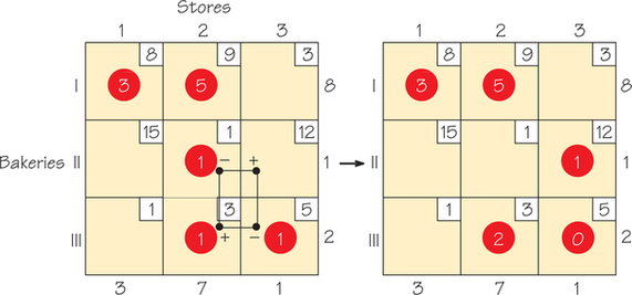
Check for yourself that the tableau on the right in Figure 4.22 with the circled entries meets the rim conditions. On the left, we show the circuit of cells with plus and minus signs (+ and −) where we have increased the amounts in the cells with + and decreased the amounts in the cells with − by 1 unit. (Note that to keep a total of five cells circled, we have set one of the circled cells to 0, because when we reduce the amounts of bread shipped in cells (II, 2) and (III, 3), we get a tie of value 0.)
We now have to ask whether this new solution is cheaper or more expensive than the one we started with. We can figure out whether this is a better or worse solution by tracking the costs of moving from the previous solution to the new one.
155
We went around a circuit where we increased a cost, decreased a cost (because we reduced the number of breads in that cell), increased a cost, and then decreased a cost before coming back to where we started, having traversed a circuit of length 4. The net effect of this collection of cost changes is . Thus, these changes, while producing a new feasible solution, give a more costly solution!
Perhaps increasing the amount shipped via a different circuit of cells would be better. Suppose we try the same process for cell (I, 3) (Figure 4.23)—that is, increase the shipping of breads from Bakery I to Store 3. To see if this is worthwhile, check the circuit formed by shipping more via cell (I, 3). It takes a bit of practice to find the circuit that this cell forms. In the case of cell (I, 3), the circuit we get is (I, 3), (I, 2), (III, 2), (III, 3), (I, 3). The cost of moving around this circuit is . We will refer to this number as the indicator value for this cell.
Indicator Value DEFINITION
The indicator value of a cell (not currently a circled cell) is the cost change associated with increasing or decreasing the amounts shipped in a circuit of cells starting at . It is computed by summing with alternating signs the costs of the cells in the circuit.
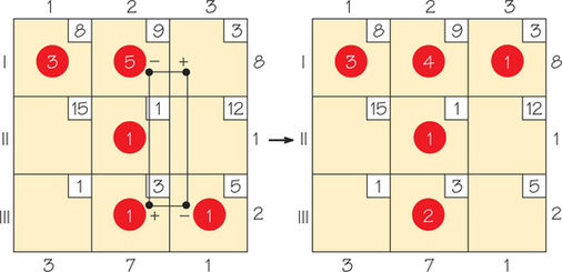
The −8 means that we can lower the cost of shipping breads by using a different pattern of meeting the demands from the supplies. We have computed the saving for shipping one bread more via cell (I, 3), but perhaps we might be able to save even more by shipping even more breads via this cell. To determine whether we could, we look at the circuit that begins at cell (I, 3). To maintain a feasible solution, we have to increase the amounts shipped via some cells of this circuit and decrease the amounts shipped via others. Because we cannot decrease the amount shipped via any cell below zero, the minimum value of any cell that must be reduced is the maximum amount that can be shipped via cell (I, 3). In this case, it means that only one bread can be shipped via cell (I, 3), thereby lowering the cost from the previous solution by 8.
When we looked to improve the solution shown in Figure 4.21 (page 153), we have now seen that by shipping via cell (I, 3), we can get a better solution. However, there might be several cells in the solution shown in Figure 4.21 that would lead to improvement. Which one should we choose? The answer is that we should adopt a greedy point of view. If there are several cells with a negative indicator value, pick the one that is “most negative” to improve the solution.
156
Given a current feasible solution (one that satisfies the rim condition), we check each cell that does not have a circled number for improvement if we ship via that cell. If a cell leads to a positive indicator value with the circuit associated with it, no improvement is possible. If a cell has a negative indicator value associated with the circuit for that cell, we can get an improvement. We select as the cell to increase that cell with the largest negative indicator value. We now have a new feasible solution that is cheaper than the one we started with and can repeat our procedure just described starting from this new feasible solution.
It turns out that there was no better cell than (I, 3) (using this greedy approach) to get an improved solution. We will take the current best solution and see if we can improve it more. It turns out that for the current tableau (Figure 4.23), all the cells have a positive indicator except for cell (III, 1):
Because the minimum of the circled numbers in the cell with a negative label is 2 in cell (III, 2), we can increase by 2 the amount shipped in cell (III, 1) and get a new solution, as shown in Figure 4.24.
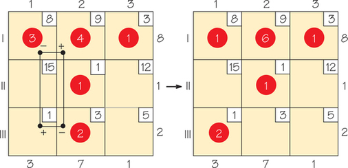
Now, for this tableau, all the empty cells have positive indicator values.
This means that the current solution is optimal. The cost of this solution is
It turns out that if all the cells associated with a feasible solution have positive indicator values, then the solution that one has reached is optimal. (Cells with a zero indicator value show that there are other solutions that achieve the same optimal value.)
How to Recognize an Optimal Solution THEOREM
We are given a transportation problem with suppliers and demanders where the amount of the supplies equals the amount of demands. A collection of circled cells is optimal (i.e., the circled cells determine a minimum cost solution) if the indicator value associated with each of the empty cells is positive. If some indicator cells are positive and some are zero, there are multiple solutions for an optimal value.
157
This theorem is the analog of the result for linear programming that states that if a corner point is feasible, and if no neighbor of the corner point has a better value of the objective function, then the corner point we are at is already an optimal one. Note that there may be other optimal solutions that use a different number of cells than , but we can never do any better in terms of the cheapness of a solution than what we have described above.
For those interested in the exciting fact that one piece of mathematics is often useful for other mathematics, we see an example of that here. The reason that an empty cell gives rise to a unique circuit with which we can try to improve the current solution of a transportation problem is the fact that when an edge not in a tree is added to a tree, it creates a unique circuit (see Chapter 3). Because we have rows and columns, a tree associated with a graph on vertices has edges, exactly the number of cells we need to fill in a transportation problem!