4 Linear Programming and the Transportation Problem

4.7 4.6 Improving on the Current Solution

Now we will describe a method guaranteed to find an optimal solution to a transportation problem.

The Stepping Stone Method DEFINITION

The stepping stone method consists of taking some feasible solution of a transportation problem and improving this solution, if it is not optimal, by shipping an additional amount using a cell with a negative indicator value.

EXAMPLE 10 Applying the Stepping Stone Method

We will work out another small example to illustrate the technique of applying the Northwest Corner Rule to get an initial solution, and then improving this solution if it is not optimal. Again, we do so by computing the indicator values of the cells and improving the current solution by shipping using a cell with a negative indicator value.

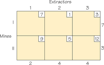
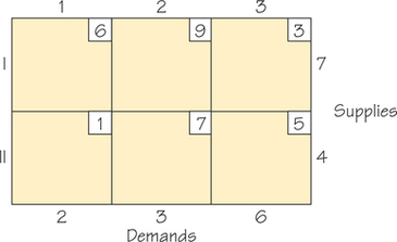
We start with an initial tableau where there are two mines that can supply ore to three companies that extract ore. There are 10 units of ore being mined and the extractors need 10 units to run at full capacity. The initial tableau for the problem is displayed in Figure 4.25.

Figure 4.25: Figure 4.25 A transportation problem where two mines supply ore to three companies that extract metal from the ore. The shipping costs are indicated.

158

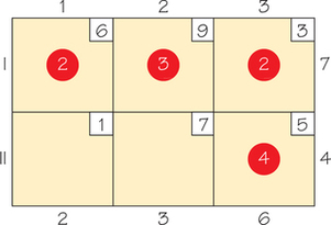
Using the Northwest Corner Rule, we find an initial feasible solution as shown in Figure 4.26. When applying the Northwest Corner Rule, we eliminate a row or column as follows: first column 1, then column 2, then row I, and we are now left with a single cell. The cost of the feasible solution shown is

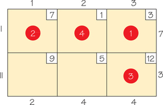
Figure 4.26: Figure 4.26 The Northwest Corner Rule has been used to find a possible way to meet the demands from the supplies for the tableau in Figure 4.25.

The two empty cells we have are (II, 1) and (II, 2). We compute the indicator value for each of these cells:

Because cell (II, 1) has a more negative indicator value, we can reduce the cost more by using that cell. increasing by 2 (because this is the minimum of circled numbers with negative signs in the computation of the indicator) the amount of metal shipped via cell (II, 1) and cell (I, 3) and reducing by 2 the amount in cells (I, 1) and (II, 3), we obtain the new tableau in Figure 4.27. This has cost

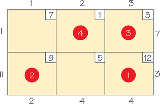
Figure 4.27: Figure 4.27 An improved solution based on the negative indicator value for cell (II, 1) in Figure 4.26.

Note that as a partial check on our work, if we multiply the indicator (−7) by 2, this is −14 and , so we reduced the cost of our first solution by 14, as expected.

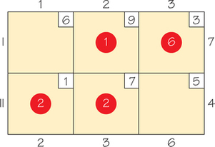
We now repeat this procedure for this new tableau. We must compute the indicator value of cells (I, 1) and (II, 2).

159

Thus, it turns out that we can increase by 1 the amount shipped by (II, 2) and get the tableau in Figure 4.28.

From this tableau, we need to compute the indicator values for the cells (I, 1) and (II, 3). We obtain

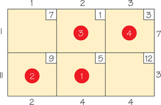
Figure 4.28: Figure 4.28 An improved solution, which turns out to be optimal, based on the negative indicator value for cell (ii, 2) in Figure 4.27.

Not surprisingly, the cell (II, 2) has a positive indicator value because in the previous tableau, that cell was the one that, when we shipped less via it, enabled us to reduce the cost. The fact that both of these indicator values are positive means that the current shipping schedule is an optimal one; that is, using a shipping schedule that ships via only four cells, we cannot find any other solution with the same value.

Self Check 3

Two dairies supply three supermarket chains with the demands for sour cream as shown in the table below. Also indicated in a cell is the cost of shipping between pairs of sites.

Use the Northwest Corner Rule to obtain a feasible solution, and compute the cost of this feasible solution.
- Applying the Northwest Corner Rule gives rise to the feasible solution shown here.
  
  The cost of this solution is 65. The indicator value for the cell (II, 1) is −7, and the indicator value for the cell (II, 2) is −4.
If the feasible solution in part (a) is not optimal, find an optimal solution.
- Consequently, this solution is not as cheap as possible. Using two iterations of the stepping stone method, we reach the following tableau, which is optimal (cost of 43).

Transportation problems arise in a very large range of situations including shipping milk from dairies to supermarkets, vegetables to health food stores, and vitamins to your local drug store. The next time you sit down to breakfast, think about how many mathematics problems were solved for you to have a healthy breakfast!