5.5 5.4 Describing Center: Mean and Median
What kind of gas mileage do you get with new cars in the Environmental Protection Agency’s "midsized cars" category? Table 5.7 gives the city and highway gas mileage (from www.fueleconomy.gov) for a representative sample of 2015 midsized cars.

| Model | City Miles per Gallon | Highway Miles per Gallon |
|---|---|---|
| Acura RDX 2WD | 20 | 28 |
| Mercedes Benz AMG S 4matic (wagon) |
15 | 21 |
| BMW 428i | 23 | 34 |
| Buick Verano | 21 | 32 |
| Chevrolet Silverado | 16 | 23 |
| Ford Fusion S | 22 | 34 |
| Infiniti QX50 | 17 | 25 |
| Kia Optima | 30 | 31 |
| Lexus GS 350 | 17 | 28 |
| Mitsubishi Galant | 26 | 31 |
| Nissan Maxima | 21 | 29 |
| Toyota Camry | 25 | 35 |
| Toyota Prius | 58 | 52 |
197
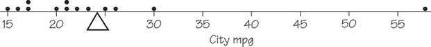
We start with graphs. Figure 5.14 is a dotplot of the city mileages of the 13 cars in the sample of midsized cars.
Dotplot DEFINITION
A dotplot is a display of the distribution of a variable in which each observation is represented by a dot above a horizontal axis. If two or more data values are the same, the dots are placed directly above each other. For large datasets, each dot may represent a specified number of observations.
Numerical summaries make the comparison that we want more specific. A numerical description of a distribution begins with a measure of its center. The two most common measures of center are the mean and the median. Basically, the mean is the arithmetic "average value" and the median is the "middle value." Sometimes the mode, the data value that occurs most frequently, is also used as a measure of center. We need to explore the precise procedures for calculating these measures and observe how they behave differently.
One way to visualize the value of the mean of a dataset is to imagine where the fulcrum would have to be placed for its dotplot to "balance." We’ve placed a triangle to mark that spot in Figure 5.14. This analogy tells us that the mean is always between the largest and smallest values, and by visual inspection, we can estimate further that the balance point appears to be somewhere between 20 and 25. Let’s see what exact value the formula yields.
Finding the Mean PROCEDURE
- Find the sum of the values.
- Divide the sum by the number of values.
If the observations are , the formula for the mean is
The common notation for the mean of all the -values is a bar over the , and is pronounced "x-bar."
EXAMPLE 9 Calculating the Mean
The mean city mileage for the 13 midsized cars in Table 5.7 is
198
We said that the Toyota Prius may be an outlier and not belong with the other cars. If we exclude the Prius, the mean city mileage drops to . The single outlier adds more than 2 mpg to the mean city mileage. This illustrates an important weakness of the mean as a measure of center: The mean is sensitive to the influence of extreme observations. These may be outliers, but a skewed distribution that has no outliers will also pull the mean toward its long tail.
We have used the middle of a distribution as an informal measure of center. The median is the formal version of the middle, with a specific rule for calculation. The median is a number where half the observations are smaller and the other half are larger.
Finding the Median PROCEDURE
- Arrange all observations (including any repeated values) in increasing order (from smallest to largest).
- If the number of observations is odd, the median is the center observation in the ordered list. To find it, start at the bottom of the ordered data values and count up observations. If the number of observations is even, the median is the mean of the two center observations in the ordered list.
EXAMPLE 10 Calculating the Median
Since we’re exploring the gas mileage cars get on the road, you might have noticed the connection that just as a median divides a road into two halves (with opposite directions of travel), a median divides a dataset into two halves! To find the median city mileage for the 2015 midsized cars, arrange the data in increasing order:
| 15 | 16 | 17 | 20 | 21 | 21 | 22 | 23 | 25 | 26 | 30 | 58 |
The median is the observation that is , or seventh from the smallest, the bold 21. Because the dataset is small, you can find this by eye—there are six observations to the left and six to the right.
What happens if we drop the Toyota Prius? The remaining 12 gas-powered cars have the following city mileages:
| 15 | 16 | 17 | 20 | 21 | 21 | 22 | 23 | 25 | 26 | 30 |
Because the number of observations is even, there is no single center observation. [In this case, .] There is a center pair of observations—the sixth and seventh observations in the ordered list, which in this case are both 21. There are five observations to the left of the pair of 21s and five to the right. The median is the mean of the center pair, which is .

You see that the median resists the influence of extreme observations better than the mean does. A very high value like the Toyota Prius is simply one observation to the right of center, and, in this case, removing it did not change the median. The Mean and Median applet (www.macmillanhighered.com/fapp10e) is an excellent way to compare the resistance of and to outliers. (Try Applet Exercise 1.)
The median and mean are the most common measures of the center of a distribution. The mean and median are close together in a roughly symmetric distribution and are equal in a perfectly symmetric distribution. In a skewed distribution, the mean is generally farther out in the long tail than is the median. For example, for the right-skewed city-miles-per-gallon data in Figure 5.14, the median is 21 mpg, while the mean (marked by the triangle) is 23.9 mpg. But that’s not the full story when it comes to the mean. As we see in Spotlight 5.2, sometimes the mean changes according to our point of view.
199
Which Mean Do You Mean? Spotlight 5.2
The word "average" can be ambiguous—sometimes used to refer to the mean, sometimes the median, and so on. But even if it is clear that we are using the mean, we still need to say what unit is the basis for our averaging. Suppose a tiny school has only 4 classrooms and their class sizes are 10, 3, 4, and 3. Most people would say this school’s "average (mean) class size" is . But that’s not how it seems to the students, half of whom are in a class twice that big! So we could find the mean from the student point of view by taking the mean of what each of the 20 students would report as the size of his or her class. This yields , a number 34% larger than 5. It turns out that the per-student mean is always at least as large as the per-class mean, which is good to know when viewing statistics about schools you are considering attending. (More information on this example can be found in Lawrence Lesser’s article "Sizing Up Class Size," in the January 2010 Mathematics Teacher.)
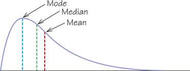
Another common numerical summary of a distribution is the mode, the most frequently occurring value in a dataset. Like the mean and median, it is a measure of location for a distribution. However, the mode is not necessarily a good measure of center. Consider a skewed distribution with its maximum height at one end and a long tail on the other, as shown in Figure 5.15. In this case, the mode, which marks the highest point, is considerably smaller than either the median or the mean and does not appear to be a good measure of the center of this distribution.
Mode DEFINITION
The mode is the most frequently occurring value in a set of numerical observations. It is possible for a dataset to have no mode, one mode, or more than one mode.
In the city-miles-per-gallon data in Table 5.7 (page 196) there are two modes, 17 and 21. Each value occurs twice in the dataset and all other values occur only once. So a distribution can have multiple modes. (The mode can also work with qualitative data: the mode for sex in Table 5.1 (page 183) is female.) We can also identify the mode(s) of a histogram. For example, Figure 5.6 (page 192) does not give the raw data of individual values for Iowa vocabulary test scores, but we can say that the modal class is grade 6.5 to 7.
200
Self Check 5
Find the mean, median, and mode of the systolic blood pressure data from Self Check 4 (page 195).
To find the mean:
To find the median, order the data from largest to smallest:
| 98 | 112 | 120 | 120 | 124 | 127 | 128 | 132 | 141 | 147 |
Since is even, find the median by taking the mean of the middle two observations: . The mode is the value that occurs most frequently. In this case, the value 120 occurs twice while all other values occur only once. Hence, the mode is 120.