8.2 8.1 Random Phenomena and Probability
343
Roll a die or choose a simple random sample (SRS) from a population. The results can’t be predicted in advance. When you roll the die, you know you will get a 1, 2, 3, 4, 5, or 6. You expect each of these outcomes to be equally likely, but you don’t know for certain which outcome will occur the next time you roll the die. An instructor chooses a random sample of three students from each class to put homework problems on the board. Because the selection is random, each possible size-3 sample is equally likely to be selected. Suppose that one day Josh comes to class without having done his homework. If the class is small, his chances of getting chosen are pretty good. On the other hand, if the class is large, he is not as likely to be in the selected sample. Josh won’t know if he will be caught unprepared for class until the sample is actually drawn.
Rolling a die and choosing a random sample are both examples of random phenomena.
Random DEFINITION
A phenomenon or trial is said to be random if individual outcomes are uncertain but the long-term pattern of many individual outcomes is predictable.
In statistics, random does not mean “haphazard.” Randomness is actually a kind of order, an order that emerges in the long run, over many repetitions. Take the example of tossing a coin. The result can’t be predicted in advance because the result will vary from coin toss to coin toss. But there is nonetheless a regular pattern in the results, a pattern that emerges clearly only after many repetitions. This remarkable fact is the basis for the idea of probability.
EXAMPLE 1 Heads Up When Tossing a Coin: Long-Run Frequency Interpretation of Probability
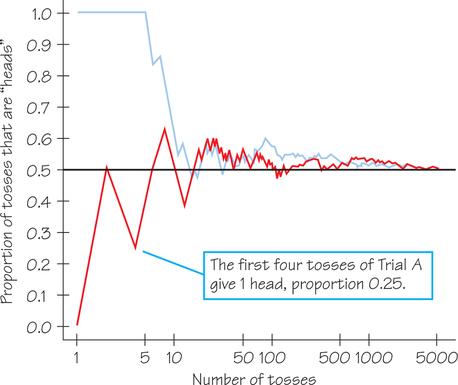
When you toss a coin, there are only two possible outcomes: heads or tails. Figure 8.3 shows the results of tossing a coin 5000 times twice. Let’s focus on Trial A, the red graph. For Trial A, the first four tosses result in tail, head, tail, tail. After four tosses, the proportion of heads is . Notice that corresponding to the first 100 tosses, there is quite a bit of fluctuation in the proportions. Now, compare the amount of fluctuation about the horizontal black line for relatively few tosses, say between 1 and 100 tosses, with the amount of fluctuation corresponding to relatively many tosses, say between 2000 and 5000 tosses. Comparatively, there is very little fluctuation in the latter interval.
Next, compare the proportions of heads for Trial A (red graph) in Figure 8.3 with those plotted for Trial B (blue graph). Trial B starts with five straight heads, so the proportion of heads is 1 until the sixth toss. Notice that the proportion of tosses that produces heads for both Trials A and B is quite variable at first. Trial A starts low and Trial B starts high. As we make more and more tosses, however, the proportions of heads for both trials get close to 0.5 and stay there. If we made yet a third trial at tossing the coin a great many times, the proportion of heads would again settle down to 0.5 in the long run. We say that 0.5 is the probability of a head. the probability 0.5 is marked by the horizontal line on the graph.
344
Probability DEFINITION
The probability of any outcome of a random phenomenon is the proportion of times the outcome would occur in a very long series of repetitions. Probabilities can be expressed as decimals, percentages, or fractions.
Algebra Review Appendix
Fractions, Percents, and Percentages

The Probability applet (see Applet Exercise 1, page 399) animates Figure 8.3. It allows you to choose the probability of a coin landing on heads and simulate a specific number of tosses of a coin with that probability. Try it. You will see that the proportion of heads gradually settles down close to the probability. Equally important, you will also see that the proportion in a small or moderate number of tosses can be far from the probability. Probability describes only what happens in the long run. Random phenomena are irregular and unpredictable in the short run.
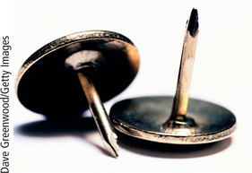
We might suspect that a coin has probability 0.5 of coming up heads just because the coin has two sides. However, such suspicions are not always correct. For example, suppose we flip a tack, which can land either point up or point down, as shown in Figure 8.4. Would the probability of the tack landing point up still be 0.5? (To find out, complete Exercise 3 on page 390.) Since probability describes what happens in a great many trials, you will need to observe the outcomes of many flips of a tack in order to pin down this probability.
Gamblers have known for centuries that the fall of coins, cards, and dice displays clear patterns in the long run. In fact, Spotlight 8.1 presents a question about a gambling game that launched probability as a formal branch of mathematics.
345
The Problem of Points Spotlight 8.1
In 1654, Antoine Gombaud, Chevalier de Méré, an amateur mathematician, posed the following problem, called the “Problem of Points”:
Two players agree to play rounds of a game of chance in which each has an equal chance of winning. They both contribute an equal amount of money to a prize. The first player to win a preset number of rounds gets the prize. Unfortunately, the game is interrupted before completion of all the rounds. The question is: How should the prize be divided fairly?
Mathematicians Blaise Pascal and Pierre de Fermat took up the challenge to solve this problem. This led to a series of correspondences between Pascal and Fermat, the content of which laid the foundation for the modern theory of probability.

In Exercise 13 (page 391), you can solve a simplified version of the “Problem of Points.”
The idea of probability rests on the observed fact that the average result of many thousands of chance outcomes can be known with near certainty. But a definition of probability as “long-run proportion” is vague. Who can say what the “long run” is? We can always toss the coin another 1000 times. Instead, we give a mathematical description of how probabilities behave, based on our understanding of long-run proportions. To see how to proceed, we return to the very simple random phenomenon of tossing a coin once.
When we toss a coin, we cannot know the outcome in advance. What do we know? We are willing to say that the outcome will be either heads or tails. We believe that each of these outcomes is equally likely, hence each has probability . This description of coin tossing has two parts:
- A list of possible outcomes
- The probability for each outcome
We will see that this description is the basis for all the probability models in Section 8.4. Here is the vocabulary we use.
Sample Space DEFINITION
The sample space of a random phenomenon is the set of all possible outcomes that cannot be broken down further into simpler components.
346
Event DEFINITION
An event is any outcome or any set of outcomes of a random phenomenon. That is, an event is a subset of the sample space. A simple event is a set of a single outcome from the sample space.
Probability Model DEFINITION
A probability model is a mathematical description of a random phenomenon consisting of two parts: a sample space and a way of assigning probabilities to events.
The sample space can be very simple or very complex. When we toss a coin once, there are two possible outcomes, heads or tails. So the sample space is . If we draw a random sample of 1000 U.S. residents that are 18 years of age or over, as opinion polls often do, the sample space contains all possible choices of 1000 of the 235 million adults in the country. This is extremely large: .
EXAMPLE 2 Tossing Two Coins: The Importance of Sample Space
Probabilities can be hard to determine without detailing or diagramming the sample space. For example, E. P. Northrop notes that even the great 18th-century French mathematician Jean le Rond d’Alembert tripped on the question “In two coin tosses, what is the probability that heads will appear at least once?” Because the number of heads could be 0, 1, or 2, d’Alembert reasoned (incorrectly) that each of those possibilities would have an equal probability of , and so he reached the (wrong) answer of .
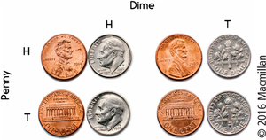
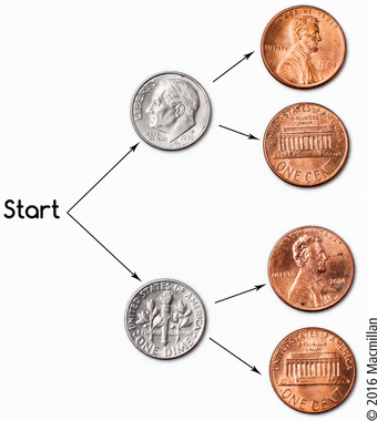
What went wrong? Well, could not be the fully detailed sample space because “1 head” can happen in more than one way. For example, if you flip a dime and a penny once apiece, you could display the sample space with a table, such as the one in Figure 8.5.
347
Another way to generate these four outcomes is with the tree diagram shown in Figure 8.6. Each possible left-to-right pathway through the branches generates an outcome. For example, going up (to dime “heads”) and then down (to penny “tails”) yields the outcome HT.
Either way, we can see that the sample space has 4, not 3, equally likely outcomes. With the table or tree diagram in view, you may already see that the correct probability of at least 1 head is not , but .
Self Check 1
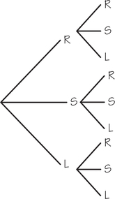
At an intersection, a driver has the choice of turning right or left or going straight (use R for right, L for left, and S for straight). You are standing at this intersection and watch the next two cars go through. Use a tree diagram to identify the sample space for the outcomes of this situation.
EXAMPLE 3 Pair-a-Dice: Outcomes for Rolling Two Dice
Rolling one six-sided die has an obvious sample space of six equally likely outcomes: . But many board games (and casino games) involve rolling two dice and noting the sum of the spots on the two sides that are facing up. We know from our experience playing games like Monopoly that the 11 possible sums are not equally likely because, for example, there are many ways to get a sum of 7 but only one way to get a sum of 12.

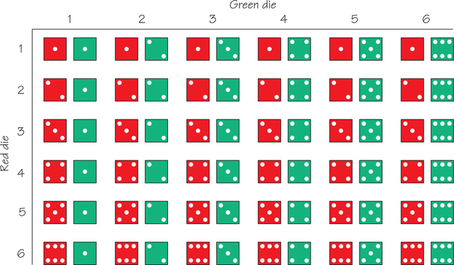
We start by identifying the sample space in order to find the exact probabilities and patterns of the various dice sums. Because of the large number of possible outcomes, the table in Figure 8.7 is a more straightforward representation of the sample space 5 than a tree diagram would be. Figure 8.7 shows possible (and equally likely) ways to roll two dice.
The longest rising diagonal of the table shows the six ways that the sum can equal 7. Therefore, it makes sense that the probability of the sum being 7 is .
348
Self Check 2
Using the table in Figure 8.7, how many possibilities are there for rolling a sum of 6? What is the probability of a sum of 6?
- Following the diagonal directly above the longest rising diagonal shows five possibilities for a sum of 6. The probability is 5/36.