8.7 8.6 Continuous Probability Models
371
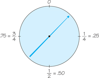
When we use the table of random digits (Table 7.1, page 298) to select a digit between 1 and 9, the discrete probability model assigns probability to each of the 10 possible outcomes. Suppose we want to choose a number at random between 0 and 1, allowing any number between 0 and 1 as the outcome. You can do this with technology, such as by using the TI-84 calculator command sequence or the Microsoft Excel spreadsheet software command = RAND(). [Recall that Spotlight 7.1 on page 300 uses RAND() to select a random sample.] You can visualize such a random number by thinking of a spinner needle (Figure 8.16) that turns freely around its center and slowly comes to a stop. The pointer can come to rest anywhere on a circle that is marked from 0 to 1.
The sample space is now an entire interval of numbers:
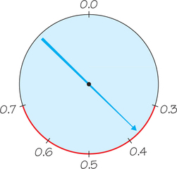
How can we assign probabilities to events such as {}? See Figure 8.17.
As in the case of selecting a random digit, we would like all possible outcomes to be equally likely. But we cannot assign probabilities to each individual value of and then sum because there are infinitely many possible values—too many to count or list. Instead, we use a second way of assigning probabilities directly to events—as areas under a curve. By Probability Rule 2, the curve must have a total area of 1 underneath it, corresponding to a total probability of 1. We call such curves density curves, which were introduced in Chapter 5 (see Example 15, page 210). We restate the definition here.
372
Density Curve DEFINITION
A density curve is a curve that
- is always on or above the horizontal axis
- has an area of exactly 1 underneath it
Continuous Probability Model DEFINITION
A continuous probability model is a probability model that assigns probabilities as areas under a density curve. The area under the curve and above any interval of values is the probability of an outcome in that interval.
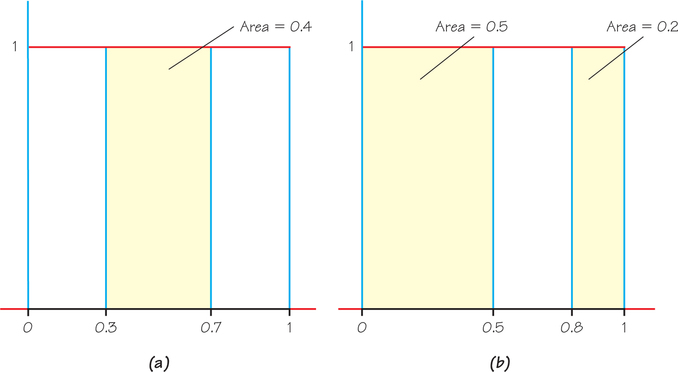
The random-number generator will spread its output uniformly across the entire interval from 0 to 1 if we allow it to generate many numbers. The results of many trials are represented by the density curve of a uniform probability model. This density curve appears in red in Figure 8.18. It has a height of 1 over the interval from 0 to 1, and a height of 0 everywhere else. The area under the density curve is 1, the area of a square with a base of 1 and height of 1. The probability of generating a number in any interval is the area above that interval and under the density curve. (This density curve showed up in Chapter 5, Exercise 73, page 238.)
As Figure 8.18a illustrates, the probability that the random-number generator produces a number between 0.3 and 0.7 inclusive is
because the rectangular area under the density curve above the interval from 0.3 to 0.7 is 0.4. (The area of a rectangle is the product of its height and length. The height of this density curve is 1, and the width of this interval is . So the area is .)
373
Also, we can apply Probability Rule 4 (addition rule for disjoint events) to non-overlapping intervals such as
The last event consists of two non-overlapping intervals, so the total area above the event is found by adding two areas, as illustrated by Figure 8.18b. This assignment of probabilities obeys all our rules for probability.
The probability model for a continuous random variable assigns probabilities to intervals of outcomes rather than to individual point outcomes. In fact, all continuous probability models assign probability 0 to every individual outcome. Only intervals of values have positive probability. To see that this is true, consider a specific outcome such as in Figure 8.18. In this example, the probability of any interval is the same as its length. The point 0.6 has no length, so this probability is 0.
EXAMPLE 18 Roundoff Error: Application of the Continuous Uniform Model
Before data values are presented, they sometimes get rounded to, say, the nearest whole number for ease of reading. For example, rounding 32.7 to 33 creates a roundoff error of , and rounding 14.17 to 14 yields a roundoff error of . Roundoff error can be critical to keep track of in data analysis and is one of many applications of the continuous uniform probability model. By rounding to the nearest whole number, the absolute value of the roundoff error cannot exceed , and it is usually assumed that each roundoff error is equally likely to be any number between −0.5 and 0.5. Note that this example shows that so long as the total area under the density curve is 1, there is no reason the horizontal axis variable has to be between 0 and 1.
Algebra Review Appendix
Rounding Numbers
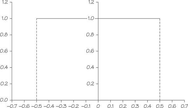
Going further, the horizontal axis variable is also not limited to an interval of length 1. For example, consider choosing a random number from the continuous interval from 1 to 3. For a rectangular area under a density curve to remain 1, a horizontal base of length would require the vertical height to be .
374
Self Check 13
Suppose you want to pick a random number from the uniform distribution over the interval from 2 to 6.
- Draw the graph of a uniform density curve on the interval from 2 to 6.
The graph of the density curve (a) along with shaded region corresponding to part (b) appears below.
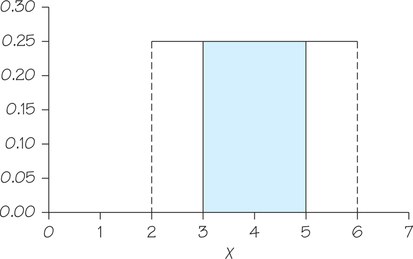
- Find the probability that a randomly selected number lies between 3 and 5. In other words, find .
The density curves that are most familiar to us are the normal curves, which were introduced in Chapter 5. Because any density curve describes an assignment of probabilities, normal distributions are continuous probability models. Recall the total area under a normal curve is 1. Let’s revisit Example 17 from Chapter 7 (page 319), using the language of probability.
EXAMPLE 19 Areas under a Normal Curve Are Probabilities
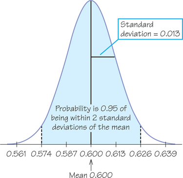
Suppose that 60% of adults agree with this statement: “Most people who want to get ahead can make it if they’re willing to work hard.” All adults form a population, with population proportion . Interview an SRS of 1500 people from this population and find the proportion of the sample who agree with the statement. We know that if we take many such samples, the statistic will vary from sample to sample according to a normal distribution, with
The 68—95—99.7 rule now gives probabilities for the value of from a single SRS. The probability is 0.95 that lies between 0.574 and 0.626 (within 2 standard deviations of the mean). Figure 8.20 shows this probability as an area under the normal density curve.
All that is new is the language of probability. “Probability is 0.95” is shorthand for “95% of the time in a very large number of samples.”