8.9 8.8 The Central Limit Theorem
The key to finding a confidence interval that estimates a population proportion (Chapter 7) is the fact that the sampling distribution of a population proportion is close to normal when the sample is large. This fact is an application of one of the most important results of probability theory, the central limit theorem. This theorem says that the distribution of any random phenomenon tends to be normal if we average it over a large number of independent repetitions. The central limit theorem allows us to analyze and predict the results of chance phenomena when we average over many observations.
Central Limit Theorem THEOREM
Draw an SRS of size from any large population with mean and finite standard deviation . Then
- The mean of the sampling distribution of is .
- The standard deviation of the sampling distribution of is .
- The central limit theorem says that the sampling distribution of is approximately normal when the sample size n is large ().
381
The first two parts of this statement can be proved from the definitions of the mean and the standard deviation. They are true for any sample size . The central limit theorem is a much deeper result. Pay attention to the fact that the standard deviation of a mean decreases as the number of observations increases. Together with the central limit theorem, this supports three general statements that help us understand a wide variety of random phenomena:
- Averages are less variable than individual observations.
- Averages are more normal than individual observations.
- Averages of large samples are less variable and more normal than averages of smaller samples.

The Central Limit Theorem applet (see Applet Exercise 4, page 399) enables you to watch the central limit theorem in action. You can select a distribution that is strongly skewed, not at all normal. As you increase the size of the sample, the distribution of the mean gets closer and closer to the normal shape.
EXAMPLE 24 Heights of Young Women
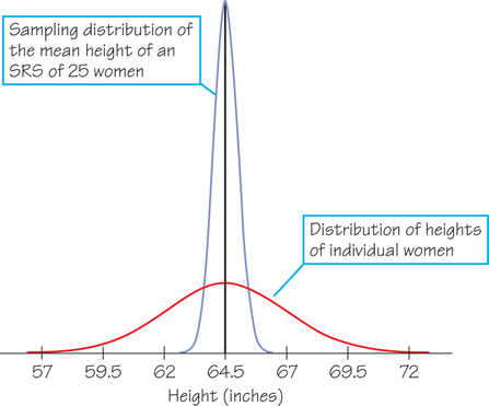
The distribution of heights of young adult women is approximately normal, with mean 64.5 inches and standard deviation 2.5 inches. This normal distribution describes the population of young women. It is also the probability model for choosing one woman at random from this population and measuring her height. For example, the 68-95-99.7 rule says that the probability is 0.95 that a randomly chosen woman is between 59.5 and 69.5 inches tall.

Now choose an SRS of 25 young women at random and take the mean of their heights. The mean varies in repeated samples; the pattern of variation is the sampling distribution of . The sampling distribution has the same center ( inches) as the population of young women. The standard deviation of the sampling distribution of is
The standard deviation describes the variation when we measure many individual women. The standard deviation of the distribution of describes the variation in the average heights of samples of women when we take many samples. The average height is less variable than individual heights.
Figure 8.24 compares the two distributions: Both are normal and both have the same mean, but the average height of 25 randomly chosen women has much less variability. For example, the 68-95-99.7 rule says that 95% of all averages lie between 63.5 and 65.5 inches because two of 's standard deviations make 1 inch. This 2-inch span is just one-fifth as wide as the 10-inch span that catches the middle 95% of heights for individual women.
382
The central limit theorem says that in large samples, the sample mean is approximately normal. In Figure 8.24, we show a normal curve for even though the sample size of 25 is not very large. Is that acceptable? How large a sample is needed for the central limit theorem to work depends on how far from a normal curve the model we start with is. The closer to normality we start, the quicker the distribution of the sample mean becomes normal. In fact, if individual observations follow a normal curve, the sampling distribution of is exactly normal for any sample size. So Figure 8.24 is accurate. The central limit theorem is a striking result because as gets large, it works for any model we may start with, no matter how far it is from normal—as you will see in Example 25.
EXAMPLE 25 Lou Gets Entertainment
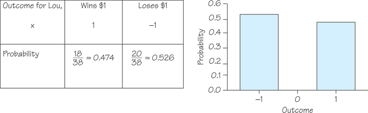
Return to Example 22 (page 378) and to Lou, who bets on red at the roulette wheel. Figure 8.25 shows the probability model and corresponding probability histogram for Lou’s favorite bet.
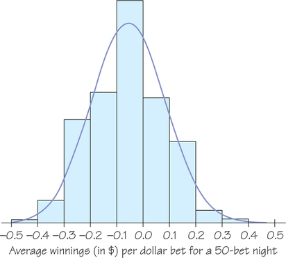
The probability model in Figure 8.25 is discrete, with just two possible outcomes: win $1 or lose $1. Yet the central limit theorem says that the average outcome of many bets follows a normal curve. Lou is a habitual gambler who places 50 bets of $1 on red almost every night. Because we know the probability model for a bet on red, we can simulate Lou’s experience over many nights at the roulette wheel. The histogram in Figure 8.26, made from a simulation of 1000 nights, shows Lou’s average winnings per bet, , from bets.
383
As the central limit theorem says, the distribution looks normal and all we need to completely specify the normal curve shown in Figure 8.26 is its mean and standard deviation. For that we return to the distribution of outcomes for one bet on red in Figure 8.25. From Example 22 (page 378) and Self Check 16 (page 380) we know that the mean and standard deviation are , respectively. Next, we use the information from the central limit theorem to specify the mean and standard deviation of the average outcome, , from bets.
Now that we have completely specified the approximate distribution of , we can apply the 99.7 part of the 68—95—99.7 rule from Section 5.9 (page 216): Almost all average nightly winnings per bet will fall within 3 standard deviations of the mean, that is, between
and
384
This gives us a 99.7% confidence interval for Lou’s mean winnings per bet, : between .
What is more interesting to Lou is not average winnings per bet, but total winnings for the whole 50-bet night. To find this out, Lou can simply multiply both endpoints from the preceding 99.7% confidence interval by 50. So Lou’s total winnings after 50 bets of $1 each will almost surely fall between
and
Each night, Lou may win as much as $18.50 or lose as much as $23.80. Note that he will usually lose more on a bad night than he will win on a good night. Some people find gambling exciting because the outcome, even after an evening of bets, is uncertain. It is possible to beat the odds and walk away a winner. It’s all a matter of luck.
The casino, however, is in a different position than individual gamblers such as Lou. It doesn’t want rollercoaster excitement, just steady income. As we’ll see from Example 26, that is exactly what they get.
EXAMPLE 26 The Casino Gets Rich
The casino bets with all its customers—perhaps 100,000 individual red/black roulette bets in a week. The central limit theorem guarantees that the distribution of average customer winnings on 100,000 bets is very close to normal. The mean, from the gambler’s point of view, is still the mean outcome for one bet, −$0.053, a loss of 5.3 cents per dollar bet. The key point is that the standard deviation is much smaller when we average over 100,000 bets. It is
Here is what the 99.7% confidence interval estimate of the average result looks like after 100,000 bets:
Because the casino covers so many bets, the standard deviation of the average winnings per bet becomes very small. Not only is the mean negative, but the entire 99.7% confidence interval is also in the negative region, so the total result is virtually certain to be in the casino’s favor. The gamblers’ losses and the casino’s winnings are almost certain to average between 4.4 and 6.2 cents for every dollar bet.
The gamblers who collectively place those 100,000 bets will lose money. The probable window of their losses is
The gamblers are almost certain to lose—and the casino is almost certain to collect—between $4400 and $6200 on those 100,000 bets. What’s more, the interval of average outcomes continues to narrow as still more bets are made. That is how a casino can make a business out of gambling.