1 Exchange Rates and Prices in the Long Run: Purchasing Power Parity and Goods Market Equilibrium
Arbitrage will force the prices of homogeneous goods in different countries to be the same, when measured in the same currency. For a single good this yields the law of one price; for a basket of goods purchasing power parity.
1. The Law of One Price
The law of one price (LOOP) asserts that, ignoring trade frictions, the price of a good must be same in different countries when expressed in the same currency. Define the real relative price of good g in Europe relative to the U.S. by 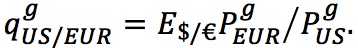 LOOP says
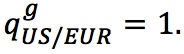
2. Purchasing Power Parity
If LOOP holds for each good, it holds for the baskets too, so qUS/EUR = E$/€ PEUR⁄PUS = 1. This is absolute purchasing power parity (PPP).
3. The Real Exchange Rate
The real exchange rate q is the relative price of the Foreign basket compared to the Home basket. If q increases, Home has a real depreciation; if q decreases, Home has a real appreciation.
4. Absolute PPP and the Real Exchange Rate
Absolute PPP implies q = 1. This is commonly used as a benchmark: If q < 1 the Foreign currency is undervalued; if q > 1, it is overvalued.
5. Absolute PPP, Prices, and the Nominal Exchange Rate
Absolute PPP implies E$/€ = PUS⁄PEUR. PPP therefore will be a key building block in our theory of exchange rate determination.
6. Relative PPP, Inflation, and Exchange Rate Depreciation
Relative PPP: the rate of depreciation equals the difference in inflation rates,  Absolute PPP implies relative PPP, but the converse does not hold.
7. Summary
PPP implies a close relationship between price levels and exchange rates.
Emphasize this difference, since students sometimes use these terms interchangeably.
Just as arbitrage occurs in the international market for financial assets, it also occurs in the international markets for goods. An implication of complete goods market arbitrage would be that the prices of goods in different countries expressed in a common currency must be equalized. Applied to a single good, this idea is called the law of one price; applied to an entire basket of goods, it is called the theory of purchasing power parity.
Why should these “laws” hold? If the price of a good is not the same in two locations, buyers will rush to buy at the cheap location (forcing prices up there) and avoid buying from the expensive location (forcing prices down there). Some factors, such as the costs of transporting goods between locations, may hinder the process of arbitrage, and more refined models take such frictions into account. For now, our goal is to develop a simple yet useful theory based on an idealized world of frictionless trade where transaction costs can be neglected. We start at the microeconomic level with single goods and the law of one price. We then move to the macroeconomic level to consider baskets of goods and purchasing power parity.
65
The Law of One Price
The law of one price (LOOP) states that in the absence of trade frictions (such as transport costs and tariffs), and under conditions of free competition and price flexibility (where no individual seller or buyer has the power to manipulate prices and prices can freely adjust), identical goods sold in different locations must sell for the same price when prices are expressed in a common currency.
To see how the law of one price operates, consider the trade in diamonds that takes place between the United States and the Netherlands. Suppose that a diamond of a given quality is priced at €5,000 in the Amsterdam market, and the exchange rate is $1.20 per euro. If the law of one price holds, the same-quality diamond should sell in New York for (€5,000 per diamond) × (1.20 $/€) = $6,000 per diamond.
Point out this argument is identical to the argument for spot arbitrage in the last chapter: In fact spot arbitrage is LOOP applied to spot contracts. But go through the same two-step derivation of the arbitrage condition.
Why will the prices be the same? Under competitive conditions and frictionless trade, arbitrage will ensure this outcome. If diamonds were more expensive in New York, arbitragers would buy at a low price in Holland and sell at a high price in Manhattan. If Dutch prices were higher, arbitragers would profit from the reverse trade. By definition, in a market equilibrium there are no arbitrage opportunities. If diamonds can be freely moved between New York and Amsterdam, both markets must offer the same price. Economists refer to this situation in the two locations as an integrated market.
We can mathematically state the law of one price as follows, for the case of any good g sold in two locations, say, Europe (EUR, meaning the Eurozone) and the United States (US). The relative price (denoted  ) is the ratio of the good’s price in Europe relative to the good’s price in the United States where both prices are expressed in a common currency.
Make students think through the units of measurement of all these terms, in order to see that the two sides are actually commensurate.
Using subscripts to indicate locations and currencies, the relative price can be written
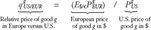
where  is the good’s price in the United States,
  is the good’s price in Europe, and E$/€ is the dollar-euro exchange rate used to convert euro prices into dollar prices.
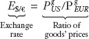
Notice that  expresses the rate at which goods can be exchanged: it tells us how many units of the U.S. good are needed to purchase one unit of the same good in Europe (hence, the subscript uses the notation US/EUR). This contrasts with the nominal exchange rate E$/€ which expresses the rate at which currencies can be exchanged ($/€).
This is a nice place to mention empirical evidence on the failure of LOOP, say the Engel-Rogers evidence about prices in Canadian and U.S. cities. It is also fun to talk about border effects, although this will appear much later in the book.
The law of one price may or may not hold. Recall from Chapter 13 that there are three possibilities in an arbitrage situation of this kind: the ratio exceeds 1 and the good is costlier in Europe; the ratio is less than 1 and the good is cheaper in Europe; or 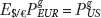 , the ratio is
  , and the good is the same price in both locations. Only in the final case is there no arbitrage, the condition that defines market equilibrium. In equilibrium, European and U.S. prices, expressed in the same currency, are equal; the relative price q equals 1, and the law of one price holds.
66
How does the law of one price further our understanding of exchange rates? We can rearrange the equation for price equality, 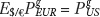 , to show that if the law of one price holds, then the exchange rate must equal the ratio of the goods’ prices expressed in the two currencies:
One final word of caution: given our concerns in the previous chapter about the right way to define the exchange rate, we must take care when using expressions that are ratios to ensure that the units on each side of the equation correspond. In the last equation, we know we have it right because the left-hand side is expressed in dollars per euro and the right-hand side is also a ratio of dollars to euros ($ per unit of goods divided by € per unit of goods).
Purchasing Power Parity
The principle of purchasing power parity (PPP) is the macroeconomic counterpart to the microeconomic law of one price (LOOP). The law of one price relates exchange rates to the relative prices of an individual good, while purchasing power parity relates exchange rates to the relative prices of a basket of goods. In studying international macroeconomics, purchasing power parity is the more relevant concept.
This may seem trivial, but it often helps to derive this by writing down price indices defined over two goods, and then imposing LOOP.
We can define a price level (denoted P) in each location as a weighted average of the prices of all goods g in a basket, using the same goods and weights in both locations. Let PUS be the basket’s price in the United States and PEUR the basket’s price in Europe. If the law of one price holds for each good in the basket, it will also hold for the price of the basket as a whole.1
Again, make sure they understand the units with which q is measured.
To express PPP algebraically, we can compute the relative price of the two baskets of goods in each location, denoted qUS/EUR:

Just as there were three possible outcomes for the law of one price, there are three possibilities for PPP: the basket is cheaper in United States; the basket is cheaper in Europe; or E$/€PEUR = PUS; the basket is the same price in both locations, and qUS/EUR = 1. In the first two cases, the basket is cheaper in one location and profitable arbitrage on the baskets is possible. Only in the third case is there no arbitrage. PPP holds when price levels in two countries are equal when expressed in a common currency. This statement about equality of price levels is also called absolute PPP.
67
For example, suppose the European basket costs €100, and the exchange rate is $1.20 per euro. For PPP to hold, the U.S. basket would have to cost 1.20 × 100 = $120.
The Real Exchange Rate
Say that just as the nominal exchange rate is the relative price of foreign currency in terms of domestic currency, so too is the real exchange rate, the relative price of (a basket of) foreign goods in terms of domestic goods.
The relative price of the two countries’ baskets (denoted q) is the macroeconomic counterpart to the microeconomic relative price of individual goods (qg). The relative price of the baskets is one of the most important variables in international macroeconomics, and it has a special name: it is known as the real exchange rate. The real exchange rate qUS/EUR = E$/€ PEUR/PUS tells us how many U.S. baskets are needed to purchase one European basket.
As with the nominal exchange rate, we need to be careful about what is in the numerator of the real exchange rate and what is in the denominator. According to our definition (based on the case we just examined), we will refer to qUS/EUR = E$/€ PEUR/PUS as the home country, or the U.S. real exchange rate: it is the price of the European basket in terms of the U.S. basket (or, if we had a Home-Foreign example, the price of a Foreign basket in terms of a Home basket).
To avoid confusion, it is essential to understand the difference between nominal exchange rates (which we have studied so far) and real exchange rates. The exchange rate for currencies is a nominal concept; it says how many dollars can be exchanged for one euro. The real exchange rate is a real concept; it says how many U.S. baskets of goods can be exchanged for one European basket.
Similarly, real devaluations and revaluations
The real exchange rate has some terminology similar to that used with the nominal exchange rate:
- If the real exchange rate rises (more Home goods are needed in exchange for Foreign goods), we say Home has experienced a real depreciation.
- If the real exchange rate falls (fewer Home goods are needed in exchange for Foreign goods), we say Home has experienced a real appreciation.
Absolute PPP and the Real Exchange Rate
We can restate absolute PPP in terms of real exchange rates: purchasing power parity states that the real exchange rate is equal to 1. Under absolute PPP, all baskets have the same price when expressed in a common currency, so their relative price is 1.
Construct numerical examples and ask whether the currency is undervalued or overvalued.
It is common practice to use the absolute PPP-implied level of 1 as a benchmark or reference level for the real exchange rate. This leads naturally to some new terminology:
- If the real exchange rate qUS/EUR is below 1 by x%, then Foreign goods are relatively cheap: x% cheaper than Home goods. In this case, the Home currency (the dollar) is said to be strong, the euro is weak, and we say the euro is undervalued by x%.
- If the real exchange rate qUS/EUR is above 1 by x%, then Foreign goods are relatively expensive: x% more expensive than Home goods. In this case, the Home currency (the dollar) is said to be weak, the euro is strong, and we say the euro is overvalued by x%.
For example, if a European basket costs E$/€ PEUR = $550 in dollar terms, and a U.S. basket costs only PUS = $500, then qUS/EUR = E$/€ PEUR/PUS = $550/$500 = 1.10, the euro is strong, and the euro is 10% overvalued against the dollar.
68
Absolute PPP, Prices, and the Nominal Exchange Rate
Say that this is oldest and most basic theory of exchange rate determination. The next step will be explaining where the price levels come from. The box below makes this very clear.
Finally, just as we did with the law of one price, we can rearrange the no-arbitrage equation for the equality of price levels, E$/€PEUR = PUS, to allow us to solve for the exchange rate that would be implied by absolute PPP:

This is one of the most important equations in our course of study because it shows how PPP (or absolute PPP) makes a clear prediction about exchange rates: Purchasing power parity implies that the exchange rate at which two currencies trade equals the relative price levels of the two countries.
For example, if a basket of goods costs $460 in the United States and the same basket costs €400 in Europe, the theory of PPP predicts an exchange rate of $460/€400 = $1.15 per euro.
Thus, if we know the price levels in different locations, we can use PPP to determine an implied exchange rate, subject to all of our earlier assumptions about frictionless trade, flexible prices, free competition, and identical goods. The PPP relationship between the price levels in two countries and the exchange rate is therefore a key building block in our theory of how exchange rates are determined, as shown in Figure 14-1. Moreover, the theory is not tied to any point in time: if we can forecast future price levels, then we can also use PPP to forecast the expected future exchange rate implied by those forecasted future price levels, which is the main goal of this chapter.

Relative PPP, Inflation, and Exchange Rate Depreciation
PPP in its absolute PPP form involves price levels, but in macroeconomics we are often more interested in the rate at which price levels change than we are in the price levels themselves. The rate of growth of the price level is known as the rate of inflation, or simply inflation. For example, if the price level today is 100, and one year from now it is 103.5, then the rate of inflation is 3.5% (per year). Because inflation is such an important variable in macroeconomics, we examine the implications of PPP for the study of inflation.
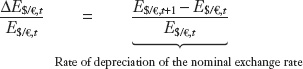
To consider changes over time, we introduce a subscript t to denote the time period, and calculate the rate of change of both sides of Equation (3-1) from period t to period t + 1. On the left-hand side, the rate of change of the exchange rate in Home is the rate of exchange rate depreciation in Home given by 2
69
Define the inflation rates separately first, rather than defining them after deriving relative PPP.
On the right of Equation (14-1), the rate of change of the ratio of two price levels equals the rate of change of the numerator minus the rate of change of the denominator:3
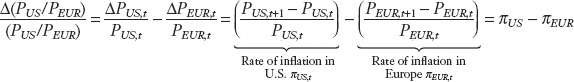
where the terms in brackets are the inflation rates in each location, denoted πUS and πEUR, respectively.
If Equation (3-1) holds for levels of exchange rates and prices, then it must also hold for rates of change in these variables. By combining the last two expressions, we obtain

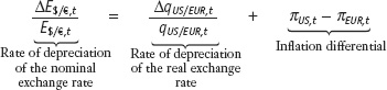
This way of expressing PPP is called relative PPP, and it implies that the rate of depreciation of the nominal exchange rate equals the difference between the inflation rates of two countries (the inflation differential).
We saw relative PPP in action in the example at the start of this chapter. Over 20 years, Canadian prices rose 16% more than U.S. prices, and the Canadian dollar depreciated 16% against the U.S. dollar. Converting these to annual rates, Canadian prices rose by 0.75% per year more than U.S. prices (the inflation differential), and the loonie depreciated by 0.75% per year against the dollar. Relative PPP held in this case.4
Point out that this makes Absolute PPP a stronger empirical hypothesis than Relative PPP.
Two points should be kept in mind about relative PPP. First, unlike absolute PPP, relative PPP predicts a relationship between changes in prices and changes in exchange rates, rather than a relationship between their levels. Second, remember that relative PPP is derived from absolute PPP. Hence, the latter always implies the former: if absolute PPP holds, this implies that relative PPP must hold also. But the converse need not be true: relative PPP does not necessarily imply absolute PPP (if relative PPP holds, absolute PPP can hold or fail). For example, imagine that all goods consistently cost 20% more in country A than in country B, so absolute PPP fails; however, it still can be the case that the inflation differential between A and B (say, 5%) is always equal to the rate of depreciation (say, 5%), so relative PPP will still hold.
70
Summary
The purchasing power parity theory, whether in the absolute PPP or relative PPP form, suggests that price levels in different countries and exchange rates are tightly linked, either in their absolute levels or in the rates at which they change. To assess how useful this theory is, let’s look at some empirical evidence to see how well the theory matches reality. We can then reexamine the workings of PPP and reassess its underlying assumptions.
PPP works well over long periods, but not over short horizons. Convergence to PPP takes a long time: The half-life of a deviation from PPP is about four years. Why would PPP fail? Transactions costs, non-traded goods, imperfect competition and legal obstacles, and price stickiness.
Evidence for PPP in the Long Run and Short Run
Is there evidence for PPP? The data offer some support for relative PPP most clearly over the long run, when even moderate inflation mounts and leads to large cumulative changes in price levels and, hence, substantial cumulative inflation differentials.
The scatterplot in Figure 14-2 shows average rates of depreciation and inflation differentials for a sample of countries compared with the United States over three decades from 1975 to 2005. If relative PPP were true, then the depreciation of each country’s currency would exactly equal the inflation differential, and the data would line up on the 45-degree line. We see that this is not literally true, but the correlation is close. Relative PPP is an approximate, useful guide to the relationship between prices and exchange rates in the long run, over horizons of many years or decades.

71
But the purchasing power theory turns out to be a fairly useless theory in the short run, over horizons of just a few years. This is easily seen by examining the time series of relative price ratio and exchange rates for any pair of countries, and looking at the behavior of these variables from year to year and not just over a long period. If absolute PPP held at all times, then the exchange rate would always equal the relative price ratio. Figure 14-3 shows 35 years of data for the United States and United Kingdom from 1975 to 2010. This figure confirms the relevance of absolute and relative PPP in the long run because the price-level ratio and the exchange rate have similar levels and drift together along a common trend. In the short run, however, the two series show substantial and persistent differences. In any given year the differences can be 10%, 20%, or more. These year-to-year differences in levels and changes show that absolute and relative PPP fail in the short run. For example, from 1980 to 1985, the pound depreciated by 45% (from $2.32 to $1.28 per pound), but the cumulative inflation differential over these five years was only 9%.
Emphasize that (1) PPP works well in the long run, but poorly in the short run, and (2) convergence to PPP is VERY slow (with a half-life of four years or so).

How Slow Is Convergence to PPP?
If PPP were taken as a strict proposition for the short run, then price adjustment via arbitrage would occur fully and instantaneously, rapidly closing the gap between common-currency prices in different countries for all goods in the basket. This doesn’t happen. The evidence suggests that PPP works better in the long run. But how long is the long run?
Research shows that price differences—the deviations from PPP—can be persistent. Estimates suggest that these deviations may die out at a rate of about 15% per year. This kind of measure is often called a speed of convergence: in this case, it implies that after one year, 85% (0.85) of an initial price difference persists; compounding, after two years, 72% of the gap persists (0.72 = 0.852); and after four years, 52% (0.52 = 0.854). Thus, approximately half of any PPP deviation still remains after four years: economists would refer to this as a four-year half-life.
72
Such estimates provide a rule of thumb that is useful as a guide to forecasting real exchange rates. For example, suppose the home basket costs $100 and the foreign basket $90, in home currency. Home’s real exchange rate is 0.900, and the home currency is overvalued, with foreign goods less expensive than home goods. The deviation of the real exchange rate from the PPP-implied level of 1 is −10% (or −0.1). Our rule of thumb tells us that next year 15% of this deviation will have disappeared (i.e., 0.015), so the new deviation will be only −0.085, meaning that Home’s real exchange rate would be forecast to be 0.915 after one year and thus end up a little bit closer to 1, after a small depreciation. Similarly, after four years, all else being equal, 52% of the deviation (or 0.052) would have been erased, and the real exchange rate would by then be 0.952, only −4.8% from PPP. (See Side Bar: Forecasting When the Real Exchange Rate Is Undervalued or Overvalued.)
What Explains Deviations from PPP?
If it takes four years for even half of any given price difference to dissipate, as research has indicated, it is no surprise that PPP does not hold in the short run. But how can arbitrage take so long to eliminate price differences? Economists have found a variety of reasons why PPP fails in the short run.
Possibly discuss Balassa-Samuelson, although that won't appear until the end of the book.
Possibly mention that prices seem to adjust fairly quickly, so that the slow convergence to PPP is an anomaly: the PPP Puzzle.
- Transaction costs. Trade is not frictionless as we have assumed thus far because the costs of international transportation are significant for most goods and because some goods also bear additional costs, such as tariffs and duties, when they cross borders. By some recent estimates, transportation costs may add about 20% on average to the price of goods moving internationally, while tariffs (and other policy barriers) may add another 10%.5 Other costs arise due to the time it takes to ship goods, and the costs and time delays associated with developing distribution networks and satisfying legal and regulatory requirements in foreign markets.
- Nontraded goods. Some goods are inherently nontradable; one can think of them as having infinitely high transaction costs. Most goods and services fall somewhere between tradable and nontradable. Consider a restaurant meal; it includes traded goods, such as some raw foods, and nontraded goods, such as the work of the chef. As a result, PPP may not hold. (See Headlines: The Big Mac Index.)
- Imperfect competition and legal obstacles. Many goods are not simple undifferentiated commodities, as LOOP and PPP assume, but are differentiated products with brand names, copyrights, and legal protection. For example, consumers have the choice of cheaper generic acetaminophen or a pricier brand-name product such as Tylenol, but these are not seen as perfect substitutes. Such differentiated goods create conditions of imperfect competition because firms have some power to set the price of their good. With this kind of market power, firms can charge different prices not just across brands but also across countries (pharmaceutical companies, for example, charge different prices for drugs in different countries). This practice is possible because arbitrage can be shut down by legal threats or regulations. If you try to import large quantities of a firm’s pharmaceutical and resell them as an unauthorized distributor, you will probably hear very quickly from the firm’s lawyers and/or from the government regulators. The same would apply to many other goods such as automobiles and consumer electronics.
- Price stickiness. One of the most common assumptions of macroeconomics is that prices are “sticky” in the short run—that is, they do not or cannot adjust quickly and flexibly to changes in market conditions. PPP assumes that arbitrage can force prices to adjust, but adjustment will be slowed down by price stickiness. Empirical evidence shows that many goods’ prices do not adjust quickly in the short run. For example, in Figure 14-3, we saw that the nominal exchange rate moves up and down in a very dramatic fashion but that price levels are much more sluggish in their movements and do not fully match exchange rate changes.
How to estimate nominal depreciation using the real exchange rate and knowledge of the speed of convergence to PPP
Forecasting When the Real Exchange Rate Is Undervalued or Overvalued
When relative PPP holds, forecasting exchange rate changes is simple: just compute the inflation differential. But how do we forecast when PPP doesn’t hold, as is often the case? Even if the real exchange rate is not equal to 1, knowing the real exchange rate and the convergence speed may still allow us to construct a forecast of real and nominal exchange rates.
To see how, let’s take an example. Start with the definition of the real exchange rate: qUS/EUR = E$/€PEUR/PUS. Rearranging, we find E$/€ = qUS/EUR × (PUS/PEUR). By taking the rate of change of that expression, we find that the rate of change of the nominal exchange rate equals the rate of change of the real exchange rate plus home inflation minus foreign inflation:
When the real exchange rate q is constant, the first term on the right is zero and we are back to the simple world of relative PPP and Equation (3-2). For forecasting purposes, the predicted nominal depreciation is then just the second term on the right, the inflation differential. For example, if the forecast is for U.S. inflation to be 3% next year and for European inflation to be 1%, then the inflation differential is +2% and we would forecast a U.S. dollar depreciation, or rise in E$/€, of +2% next year.
What if q isn’t constant and PPP fails? If there is currently a deviation from absolute PPP, but we still think that there will be convergence to absolute PPP in the long run, the first term on the right of the formula is not zero and we can estimate it given the right information.
To continue the example, suppose you are told that a U.S. basket of goods currently costs $100, but the European basket of the same goods costs $130. You would compute a U.S. real exchange rate qUS/EUR of 1.30 today. But what will it be next year? If you expect absolute PPP to hold in the long run, then you expect that the U.S. real exchange rate will move toward 1. How fast? At this point, you need to know the convergence speed. Using the 15% rule of thumb, you estimate that 15% of the 0.3 gap between 1 and 1.3 (i.e., 0.045) will dissipate over the coming year. Hence, you forecast that the U.S. real exchange will fall from 1.3 to 1.255, implying a change of −3.46% in the coming year. In this case, adding the two terms on the right of the expression given previously, you forecast that the approximate change in E next year will be the change in qUS/EUR of −3.46% plus the inflation differential of +2%, for a total of −1.46%; that is, a dollar appreciation of 1.46% against the euro.
The intuition for the result is as follows: the U.S. dollar is undervalued against the euro. If convergence to PPP is to happen, then some of that undervaluation will dissipate over the course of the year through a real appreciation of the dollar (predicted to be 3.46%). That real appreciation can be broken down into two components:
- U.S. goods will experience higher inflation than European goods (we have predicted that the inflation differential will be +2%).
- The remainder of the real appreciation will be accomplished via a 1.46% nominal dollar appreciation (predicted based on a convergence speed of 15% per year).
74
Despite these problems, the evidence suggests that as a long-run theory of exchange rates, PPP is still a useful approach.6 And PPP may become even more relevant in the future as arbitrage becomes more efficient and more goods and services are traded. Years ago we might have taken it for granted that certain goods and services (such as pharmaceuticals, customer support, and health-care services) were strictly nontraded and thus not subject to arbitrage at the international level. Today, many consumers shop for pharmaceuticals overseas to save money. If you dial a U.S. software support call center, you may find yourself being assisted by an operator in another country. In some countries, citizens motivated by cost considerations may travel overseas for dental treatment, eye care, hip replacements, and other health services (so-called medical tourism or health tourism). These globalization trends may well continue.
The Big Mac Index is always fun to do in class. Have them find more current articles on it in The Economist.
Using the Big Mac Index to measure over- and undervaluation
The Big Mac Index
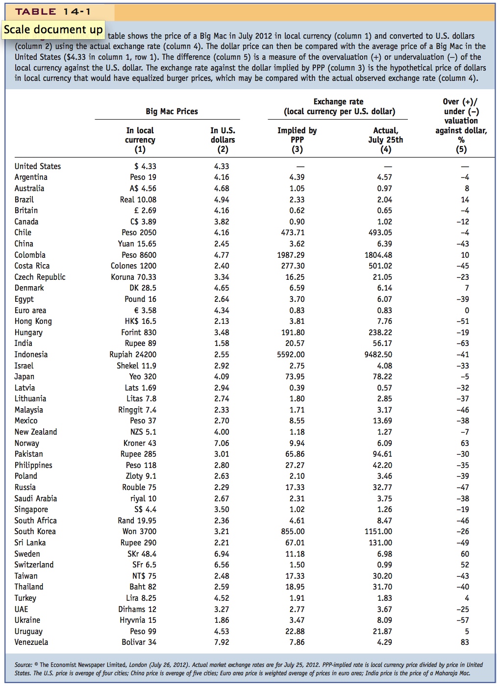
For more than 25 years, The Economist newspaper has engaged in a whimsical attempt to judge PPP theory based on a well-known, globally uniform consumer good: McDonald’s Big Mac. The over- or undervaluation of a currency against the U.S. dollar is gauged by comparing the relative prices of a burger in a common currency, and expressing the difference as a percentage deviation from one:
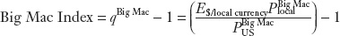

Table 14-1 shows the July 2012 survey results, and some examples will illustrate how the calculations work. Row 1 shows the average U.S. dollar price of the Big Mac of $4.33. An example of undervaluation appears in Row 2, where we see that the Buenos Aires correspondent found the same burger cost 19 pesos, which, at an actual exchange rate of 4.57 pesos per dollar, worked out to be $4.16 in U.S. currency, or 4% less than the U.S. price. So the peso was 4% undervalued against the U.S. dollar according to this measure, and Argentina’s exchange rate would have had to appreciate to 4.39 pesos per dollar to attain the level implied by a burger-based PPP theory. An example of overvaluation appears in Row 4, in the case of neighboring Brazil. There a Big Mac cost 10.08 reais, or $4.94 in U.S. currency at the prevailing exchange rate of 2.04 reais per dollar, making the Brazilian burgers 14% more expensive than their U.S. counterparts. To get to its PPP-implied level, and put the burgers at parity, Brazil’s currency would have needed to depreciate to 2.33 reais per dollar. Looking through the table, burger disparity is typical, with only 7 countries coming within ±5% of PPP.
75
76