2 Money, Prices, and Exchange Rates in the Long Run: Money Market Equilibrium in a Simple Model
PPP says price levels determine the exchange rate.
What determines price levels? In the long run, the demand and supply of money.
1. What Is Money?
Money as store of value, unit of account, and medium of exchange
2. The Measurement of Money
Define currency, M0, M1, and M2; for our purposes M is M1.
3. The Supply of Money
For simplicity, ignore deposit creation. Just assume the central bank can control M.
4. The Demand for Money: A Simple Model
Quantity theory: 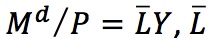 constant.
5. Equilibrium in the Money Market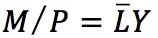
6. A Simple Monetary Model of Prices
For the U.S., 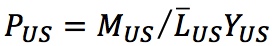 and for Europe
 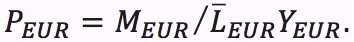 . So money growth causes a proportional increase in prices.
7. A Simple Monetary Model of the Exchange Rate
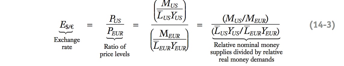
From PPP and the preceding 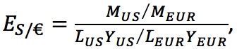 the fundamental equation of the monetary approach. Implications: (1) If MUS doubles, so will E$/€ U.S. money growth depreciates the dollar. (2) If YUS increases, E$/€ decreases; U.S. real growth appreciates the dollar.
8. Money, Growth, Inflation, and Depreciation
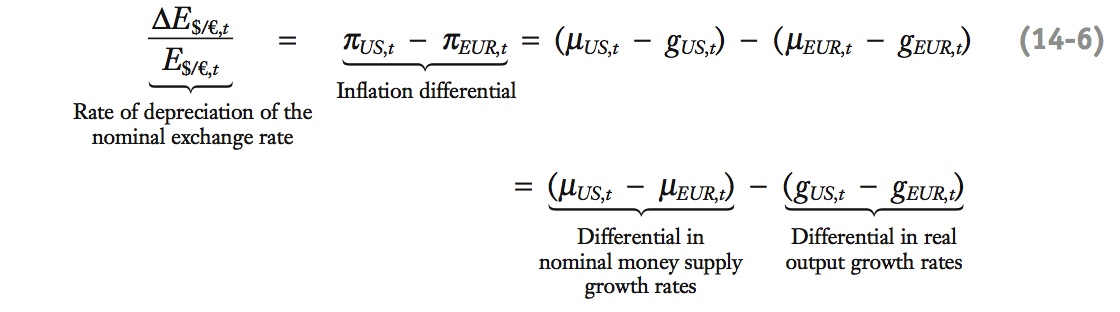
Expressed in growth rates, the fundamental equation predicts  Implications: (1) If U.S. money grows faster than European, the dollar will depreciate. (2) If the U.S. grows faster than Europe, the dollar will appreciate.
It is time to take stock of the theory developed so far in this chapter. Up to now, we have concentrated on PPP, which says that in the long run the exchange rate is determined by the ratio of the price levels in two countries. But this prompts a question: What determines those price levels?
Monetary theory supplies an answer: according to this theory, in the long run, price levels are determined in each country by the relative demand and supply of money. You may recall this theory from previous macroeconomics courses in the context of a closed economy. This section recaps the essential elements of monetary theory and shows how they fit into our theory of exchange rates in the long run.
What Is Money?
Students are probably pretty familiar with these from their Principles classes, so don't waste much time on it.
We recall the distinguishing features of this peculiar asset that is so central to our everyday economic life. Economists think of money as performing three key functions in an economy:
- Money is a store of value because, as with any asset, money held from today until tomorrow can still be used to buy goods and services in the future. Money’s rate of return is low compared with many other assets. Because we earn no interest on it, there is an opportunity cost to holding money. If this cost is low, we hold money more willingly than other assets (stocks, bonds, and so forth).
- Money is a unit of account in which all prices in the economy are quoted. When we enter a store in France, we expect to see the prices of goods to read something like “100 euros”—not “10,000 Japanese yen” or “500 bananas,” even though, in principle, the yen or the banana could also function as a unit of account in France (bananas would, however, be a poor store of value).
- Money is a medium of exchange that allows us to buy and sell goods and services without the need to engage in inefficient barter (direct swaps of goods). The ease with which we can convert money into goods and services is a measure of how liquid money is compared with the many illiquid assets in our portfolios (such as real estate). Money is the most liquid asset of all.
The Measurement of Money
You may need to review what base money is, but avoid getting into a detailed discussion of the money multiplier.
What counts as money? Clearly, currency (coins and bills) in circulation is money. But do checking accounts count as money? What about savings accounts, mutual funds, and other securities? Figure 14-4 depicts the most widely used measures of the money supply and illustrates their relative magnitudes with recent data from the United States. The most basic concept of money is currency in circulation (i.e., in the hands of the nonbank public). After that, M0 is typically the narrowest definition of money (also called “base money”), and it includes both currency in circulation and the reserves of commercial banks (liquid cash held in their vaults or on deposit at the Fed). Normally, in recent years, banks’ reserves have been very small and so M0 has been virtually identical to currency in circulation. This changed dramatically after the financial crisis of 2008 gave rise to liquidity problems, and banks began to maintain huge reserves at the Fed as a precaution. (When and how this unprecedented hoard of cash will be unwound remains to be seen, and this is a matter of some concern to economists and policy makers.)

77
A different narrow measure of money, M1, includes currency in circulation plus highly liquid instruments such as demand deposits in checking accounts and traveler’s checks, but it excludes bank’s reserves, and thus may be a better gauge of money available for transactions purposes. A much broader measure of money, M2, includes slightly less liquid assets such as savings and small time deposits.7
For our purposes, money is defined as the stock of liquid assets that are routinely used to finance transactions, as implied by the “medium of exchange” function of money. So, in this book, when we speak of money (denoted M), we will generally mean M1 (currency in circulation plus demand deposits). Many important assets are excluded from M1, including longer-term assets held by individuals and the voluminous interbank deposits used in the foreign exchange market discussed in the previous chapter. These assets do not count as money in the sense we use the word because they are relatively illiquid and not used routinely for transactions.
The Supply of Money
Ditto
How is the supply of money determined? In practice, a country’s central bank controls the money supply. Strictly speaking, by issuing notes and coins (and private bank reserves), the central bank controls directly only the level of M0, or base money, the amount of currency and reserves in the economy. However, it can indirectly control the level of M1 by using monetary policy to influence the behavior of the private banks that are responsible for checking deposits. The intricate mechanisms by which monetary policy affects M1 are beyond the scope of this book. For our purposes, we make the simplifying assumption that the central bank’s policy tools are sufficient to allow it to control the level of M1 indirectly, but accurately.8
78
The Demand for Money: A Simple Model
A simple theory of household money demand is motivated by the assumption that the need to conduct transactions is in proportion to an individual’s income. For example, if an individual’s income doubles from $20,000 to $40,000, we expect his or her demand for money (expressed in dollars) to double also.
Moving from the individual or household level up to the aggregate or macroeconomic level, we can infer that the aggregate money demand will behave similarly. All else equal, a rise in national dollar income (nominal income) will cause a proportional increase in transactions and, hence, in aggregate money demand.
Actually, this is the Cambridge (Marshallian) version of the quantity theory.
This insight suggests a simple model in which the demand for money is proportional to dollar income. This model is known as the quantity theory of money:
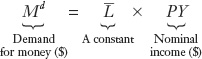
Here, PY measures the total nominal dollar value of income in the economy, equal to the price level P times real income Y. The term  is a constant that measures how much demand for liquidity is generated for each dollar of nominal income. To emphasize this point, we assume for now that every $1 of nominal income requires $ of money for transactions purposes and that this relationship is constant. (Later, we relax this assumption.)
The intuition behind the last equation is as follows: If the price level rises by 10% and real income is fixed, we are paying a 10% higher price for all goods, so the dollar cost of transactions rises by 10%. Similarly, if real income rises by 10% but prices stay fixed, the dollar amount of transactions will rise by 10%. Hence, the demand for nominal money balances, Md, is proportional to the nominal income PY.
Another way to look at the quantity theory is to convert all quantities into real quantities by dividing the previous equation by P, the price level (the price of a basket of goods). Quantities are then converted from nominal dollars to real units (specifically, into units of baskets of goods). These conversions allow us to derive the demand for real money balances:
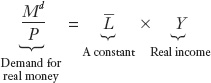
Real money balances measure the purchasing power of the stock of money in terms of goods and services. The expression just given says that the demand for real money balances is proportional to real income. The more real income we have, the more real transactions we have to perform, and the more real money we need.
79
Equilibrium in the Money Market
The condition for equilibrium in the money market is that the demand for money Md must equal the supply of money M, which we assume to be under the control of the central bank. Imposing this condition on the last two equations, we find that nominal money supply equals nominal money demand:

and, equivalently, that real money supply equals real money demand:

A Simple Monetary Model of Prices
We are now in a position to put together a simple model of the exchange rate, using two building blocks. The first building block, the quantity theory, is a model that links prices to monetary conditions. The second building block, PPP, is a model that links exchange rates to prices.
We consider two locations, or countries, as before; the United States will be the home country and we will treat the Eurozone as the foreign country. We shall refer to the Eurozone, or more simply Europe, as a country in this and later examples. The model generalizes to any pair of countries or locations.
Emphasize that in the quantity theory we are assuming income is exogenous, since prices are flexible.
Let’s consider the last equation given and apply it to the United States, adding U.S. subscripts for clarity. We can rearrange this formula to obtain an expression for the U.S. price level:

Note that the price level is determined by how much nominal money is issued relative to the demand for real money balances: the numerator on the right-hand side MUS is the total supply of nominal money; the denominator  is the total demand for real money balances.
The analogous expression for the European price level is:
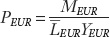
The last two equations are examples of the fundamental equation of the monetary model of the price level. Two such equations, one for each country, give us another important building block for our theory of prices and exchange rates as shown in Figure 14-5.

"Inflation is always and everywhere a monetary phenomenon"
In the long run, we assume prices are flexible and will adjust to put the money market in equilibrium. For example, if the amount of money in circulation (the nominal money supply) rises, say, by a factor of 100, and real income stays the same, then there will be “more money chasing the same quantity of goods.” This leads to inflation, and in the long run, the price level will rise by a factor of 100. In other words, we will be in the same economy as before except that all prices will have two zeros tacked on to them.
80
A Simple Monetary Model of the Exchange Rate
A long-run model of the exchange rate is close at hand. If we take the last two equations, which use the monetary model to find the price level in each country, and plug them into Equation (3-1), we can use absolute PPP to solve for the exchange rate:
Put Figure 14-1 and Figure 14-5 together to highlight the causal links in these propositions.
This is the fundamental equation of the monetary approach to exchange rates. By substituting the price levels from the monetary model into PPP, we have put together the two building blocks from Figures 3-1 and 3-5. The implications of this equation are as follows:
- Suppose the U.S. money supply increases, all else equal. The right-hand side increases (the U.S. nominal money supply increases relative to Europe), causing the exchange rate to increase (the U.S. dollar depreciates against the euro). For example, if the U.S. money supply doubles, then all else equal, the U.S. price level doubles. That is, a bigger U.S. supply of money leads to a weaker dollar. That makes sense—there are more dollars around, so you expect each dollar to be worth less.
- Now suppose the U.S. real income level increases, all else equal. Then the right-hand side decreases (the U.S. real money demand increases relative to Europe), causing the exchange rate to decrease (the U.S. dollar appreciates against the euro). For example, if the U.S. real income doubles, then all else equal, the U.S. price level falls by a factor of one-half. That is, a stronger U.S. economy leads to a stronger dollar. That makes sense—there is more demand for the same quantity of dollars, so you expect each dollar to be worth more.
The punch lines: (1) Domestic money growth causes depreciation. (2) Faster real growth should cause the currency to appreciate. Make sure they can explain why these hold.
81
Money Growth, Inflation, and Depreciation
The model just presented uses absolute PPP to link the level of the exchange rate to the level of prices and uses the quantity theory to link prices to monetary conditions in each country. But as we have said before, macroeconomists are often more interested in rates of change of variables (e.g., inflation) rather than levels.
Can we extend our theory to this purpose? Yes, but this task takes a little work. We convert Equation (3-3) into growth rates by taking the rate of change of each term.
The first term of Equation (3-3) is the exchange rate E$/€. Its rate of change is the rate of depreciation ΔE$/€/E$/€. When this term is positive, say, 1%, the dollar is depreciating at 1% per year; if negative, say, −2%, the dollar is appreciating at 2% per year.
The second term of Equation (3-3) is the ratio of the price levels PUS/PEUR, and as we saw when we derived relative PPP at Equation (3-2), its rate of change is the rate of change of the numerator (U.S. inflation) minus the rate of change of the denominator (European inflation), which equals the inflation differential πUS,t − πEUR,t.
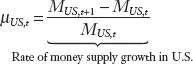
What is the rate of change of the third term in Equation (3-3)? The numerator—represents the U.S. price level, 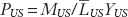 . Again, the growth rate of a fraction equals the growth rate of the numerator minus the growth rate of the denominator. In this case, the numerator is the money supply MUS, and its growth rate is μUS:
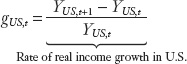
The denominator is , which is a constant  times real income YUS. Thus, grows at a rate equal to the growth rate of real income gUS:
Putting all the pieces together, the growth rate of equals the money supply growth rate μUS minus the real income growth rate gUS. We have already seen that the growth rate of PUS on the left-hand side is the inflation rate πUS. Thus, we know that

The denominator of the third term of Equation (3-3) represents the European price level, 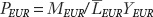 , and its rate of change is calculated similarly:

The intuition for these last two expressions echoes what we said previously: when money growth is higher than real income growth, we have “more money chasing fewer goods” and this leads to inflation.
82
Combining Equation (3-4) and Equation (3-5), we can now solve for the inflation differential in terms of monetary fundamentals and finish our task of computing the rate of depreciation of the exchange rate:
The last term here is the rate of change of the fourth term in Equation (3-3).
Equation (3-6) is the fundamental equation of the monetary approach to exchange rates expressed in rates of change, and much of the same intuition we applied in explaining Equation (3-3) carries over here.
Just say these are the same ideas, but expressed in growth rates. Also emphasize that both money growth and real growth are exogenous.
- If the United States runs a looser monetary policy in the long run measured by a faster money growth rate, the dollar will depreciate more rapidly, all else equal. For example, suppose Europe has a 5% annual rate of change of money and a 2% rate of change of real income; then its inflation would be the difference: 5% minus 2% equals 3%. Now suppose the United States has a 6% rate of change of money and a 2% rate of change of real income; then its inflation would be the difference: 6% minus 2% equals 4%. And the rate of depreciation of the dollar would be U.S. inflation minus European inflation, 4% minus 3%, or 1% per year.
- If the U.S. economy grows faster in the long run, the dollar will appreciate more rapidly, all else equal. In the last numerical example, suppose the U.S. growth rate of real income in the long run increases from 2% to 5%, all else equal. U.S. inflation equals the money growth rate of 6% minus the new real income growth rate of 5%, so inflation is just 1% per year. Now the rate of dollar depreciation is U.S. inflation minus European inflation, that is, 1% minus 3%, or −2% per year (meaning the U.S. dollar would now appreciate at 2% per year).
With a change of notation to make the United States the foreign country, the same lessons could be derived for Europe and the euro.