2 Income, Product, and Expenditure
Again, the students should be pretty familiar with all this, and the last section surveyed it. Don't get lost in the details here.
1. Three Approaches to Measuring Economic Activity
Expenditure (GNE), Product (GDP), and income (GNDI) approaches. In the closed economy GNE = GDP = GNI.
2. From GNE to GDP: Accounting for Trade in Goods and Services
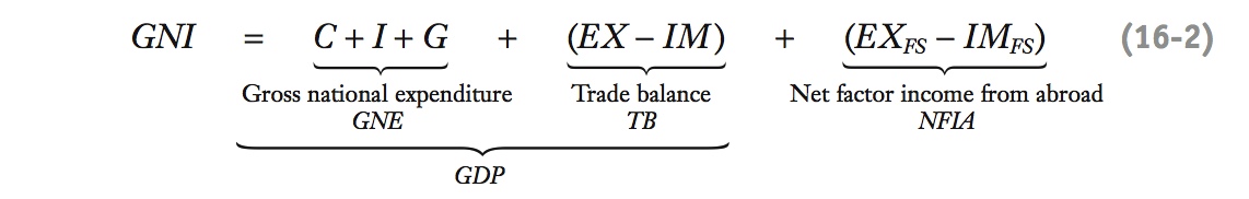
Allow for exports and imports of goods: GDP ≡ C + I + G + TB, where TB = EX – IM. If TB > 0 there is a trade surplus; if TB < 0, a trade deficit.
3. From GDP to GNI: Accounting for Trade in Factor Services
The economy exports and imports factor services. Net factor income from abroad NFIA creates income for the economy, so GNI = GDP + NFIA.
In the previous section, we sketched out all the important national and international transactions that occur in an open economy. With that overview in mind, we now formally define the key accounting concepts in the two sets of accounts and put them to use.
Three Approaches to Measuring Economic Activity
There are three main approaches to the measurement of aggregate economic activity within a country:
- The expenditure approach looks at the demand for goods: it examines how much is spent on demand for final goods and services. The key measure is gross national expenditure GNE.
- The product approach looks at the supply of goods: it measures the value of all goods and services produced as output minus the value of goods used as inputs in production. The key measure is gross domestic product GDP.
- The income approach focuses on payments to owners of factors and tracks the amount of income they receive. The key measures are gross national income GNI and gross national disposable income GNDI (which includes net transfers).
It is crucial to note that in a closed economy the three approaches generate the same number: In a closed economy, GNE = GDP = GNI. In an open economy, however, this is not true.
From GNE to GDP: Accounting for Trade in Goods and Services
As before, we start with gross national expenditure, or GNE, which is by definition the sum of consumption C, investment I, and government consumption G. Formally, these three elements are defined, respectively, as follows:
- Personal consumption expenditures (usually called “consumption”) equal total spending by private households on final goods and services, including nondurable goods such as food, durable goods such as a television, and services such as window cleaning or gardening.
- Gross private domestic investment (usually called “investment”) equals total spending by firms or households on final goods and services to make additions to the stock of capital. Investment includes construction of a new house or a new factory, the purchase of new equipment, and net increases in inventories of goods held by firms (i.e., unsold output).
- Government consumption expenditures and gross investment (often called “government consumption”) equal spending by the public sector on final goods and services, including spending on public works, national defense, the police, and the civil service. It does not include any transfer payments or income redistributions, such as Social Security or unemployment insurance payments—these are not purchases of goods or services, just rearrangements of private spending power.
As for GDP, it is by definition the value of all goods and services produced as output by firms, minus the value of all intermediate goods and services purchased as inputs by firms. It is thus a product measure, in contrast to the expenditure measure GNE. Because of trade, not all of the GNE payments go to GDP, and not all of GDP payments arise from GNE.
164
To adjust GNE and find the contribution going into GDP, we subtract the value of final goods imported (home spending that goes to foreign firms) and add the value of final goods exported (foreign spending that goes to home firms). In addition, we can’t forget about intermediate goods: we subtract the value of imported intermediates (in GDP they also count as home’s purchased inputs) and add the value of exported intermediates (in GDP they also count as home’s produced output).2 So, adding it all up, to get from GNE to GDP, we add the value of all exports denoted EX and subtract the value of all imports IM. Thus,

This important formula for GDP says that gross domestic product is equal to gross national expenditure (GNE) plus the trade balance (TB).
It is important to understand and account for intermediate goods transactions properly because trade in intermediate goods has surged in recent decades due to globalization and outsourcing. For example, according to the 2010 Economic Report of the President, estimates suggest that one-third of the growth of world trade from 1970 to 1990 was driven by intermediate trade arising from the growth of “vertically specialized” production processes (outsourcing, offshoring, etc.). More strikingly, as of 2010, it appears that—probably for the first time in world history—total world trade now consists more of trade in intermediate goods (60%) than in final goods (40%).
The trade balance TB is also called net exports. Because it is the net value of exports minus imports, it may be positive or negative.
If TB > 0, exports are greater than imports and we say a country has a trade surplus.
If TB < 0, imports are greater than imports and we say a country has a trade deficit.
In 2012, the United States had a trade deficit because exports X were $2,184 billion and imports M were $2,744 billion. Thus its trade balance was equal to −$560 billion.
From GDP to GNI: Accounting for Trade in Factor Services
Trade in factor services occurs when, say, the home country is paid income by a foreign country as compensation for the use of labor, capital, and land owned by home entities but in service in the foreign country. We say the home country is exporting factor services to the foreign country and receiving factor income in return.
165
An example of a labor service export is a home country professional temporarily working overseas, say, a U.S. architect freelancing in London. The wages she earns in the United Kingdom are factor income for the United States. An example of trade in capital services is foreign direct investment. For example, U.S.-owned factories in Ireland generate income for their U.S. owners; Japanese-owned factories in the United States generate income for their Japanese owners. Other examples of payments for capital services include income from overseas financial assets such as foreign securities, real estate, or loans to governments, firms, and households.
These payments are accounted for as additions to and subtractions from home GDP. Some home GDP is paid out as income payments to foreign entities for factor services imported by the home country IMFS. In addition, domestic entities receive some income payments from foreign entities as income receipts for factor services exported by the home country EXFS.
After accounting for these income flows, we see that gross national income (GNI), the total income earned by domestic entities, is GDP plus the factor income arriving from overseas EXFS, minus the factor income going out overseas IMFS.3 The last two terms, income receipts minus income payments, are the home country’s net factor income from abroad, NFIA = EXFS − IMFS. This may be a positive or negative number, depending on whether income receipts are larger or smaller than income payments.
With the help of the GDP expression in Equation (5-1), we obtain the key formula for GNI that says the gross national income equals gross domestic product (GDP) plus net factor income from abroad (NFIA).
In 2012 the United States received income payments from foreigners EXFS of $782 billion and made income payments to foreigners IMFS of $539 billion, so the net factor income from abroad NFIA was +$243 billion.
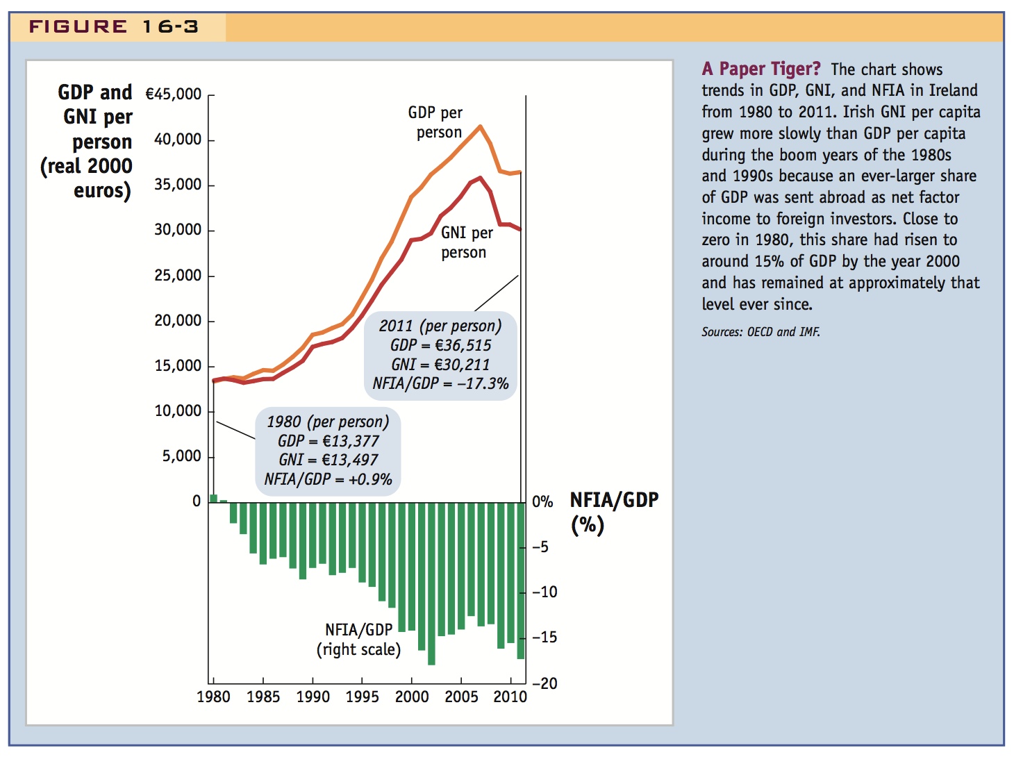
The Irish miracle raised GDP, but a lot of it went to pay factor income to foreign investors, so that the increase in income is much smaller than the increase in GDP.
Celtic Tiger or Tortoise?
International trade in factor services (as measured by NFIA) can generate a difference between the product and income measures in a country’s national accounts. In the United States, this difference is typically small, but at times NFIA can play a major role in the measurement of a country’s economic activity.
In the 1970s, Ireland was one of the poorer countries in Europe, but over the next three decades it experienced speedy economic growth with an accompanying investment boom now known as the Irish Miracle. From 1980 to 2007, Irish real GDP per person grew at a phenomenal rate of 4.1% per year—not as rapid as in some developing countries but extremely rapid by the standards of the rich countries of the European Union (EU) or the Organization for Economic Cooperation and Development (OECD). Comparisons with fast-growing Asian economies—the “Asian Tigers”—soon had people speaking of the “Celtic Tiger” when referring to Ireland. Despite a large recession after the 2008 crisis, real GDP per person in Ireland is still almost three times its 1980 level.
166
But did Irish citizens enjoy all of these gains? No. Figure 16-3 shows that in 1980 Ireland’s annual net factor income from abroad was virtually nil—about €120 per person (in year 2000 real euros) or +0.9% of GDP. Yet by 2000, and in the years since, around 15% to 20% of Irish GDP was being used to make net factor income payments to foreigners who had invested heavily in the Irish economy by buying stocks and bonds and by purchasing land and building factories on it. (By some estimates, 75% of Ireland’s industrial-sector GDP originated in foreign-owned plants in 2004.) These foreign investors expected their big Irish investments to generate income, and so they did, in the form of net factor payments abroad amounting to almost one-fifth of Irish GDP. This meant that Irish GNI (the income paid to Irish people and firms) was a lot smaller than Irish GDP.4 Ireland’s net factor income from abroad has remained large and negative ever since.
167
This example shows how GDP can be a misleading measure of economic performance. When ranked by GDP per person, Ireland was the 4th richest OECD economy in 2004; when ranked by GNI per person, it was only 17th richest.5 The Irish outflow of net factor payments is certainly an extreme case, but it serves to underscore an important point about income measurement in open economies. Any country that relies heavily on foreign investment to generate economic growth is not getting a free lunch. Irish GNI per person grew at “only” 3.6% from 1980 to the peak in 2007; this was 0.5% per year less than the growth rate of GDP per person over the same period. Living standards grew impressively, but the more humble GNI figures may give a more accurate measure of what the Irish Miracle actually meant for the Irish.
This is an interesting case to highlight the importance of net factor payments for some countries. Ask the students to think of others.
From GNI to GNDI: Accounting for Transfers of Income
4. From GNI to GNDI: Accounting for Transfers of Income
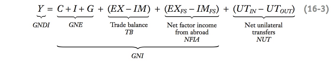
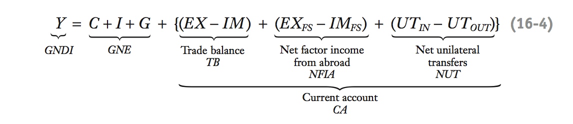
Net unilateral transfers alter disposable income: GNDI = GNI + NUT, or Y = C + I + G + TB + NFIA + NUT. GNDI is the best overall measure of the resources available to an economy.
5. What the National Economic Aggregates Tell Us
CA = TB + NFIA + NUT, so Y ≡ C + I + G + CA. Intuition: Disposable income must equal payments by home entities (GNE ≡ C + I + G) plus net payments from abroad from transactions of goods, services, and income.
6. Understanding the Data for the National Economic Aggregates
Reports data on aggregates for the U.S.
a. Some Recent Trends
C and G are fairly stable; I is more volatile. TB is the biggest part of the CA; TB deficit has grown over time. NUT is fairly small; NFIA has been consistently positive.
7. What the Current Account Tells Us
Define national saving as S = Y – C – G. This yields CA = S – I. So CA > 0 if S > I; CA < 0 if S < I. So a CA deficit means (1) we are consuming in excess of our income, or (2) we are not saving enough to finance our investment needs.
So far, we have fully described market transactions in goods, services, and income. However, many international transactions take place outside of markets. International nonmarket transfers of goods, services, and income include such things as foreign aid by governments in the form of official development assistance (ODA) and other help, private charitable gifts to foreign recipients, and income remittances sent to relatives or friends in other countries. These transfers are “gifts” and may take the form of goods and services (food aid, volunteer medical services) or income transfers.
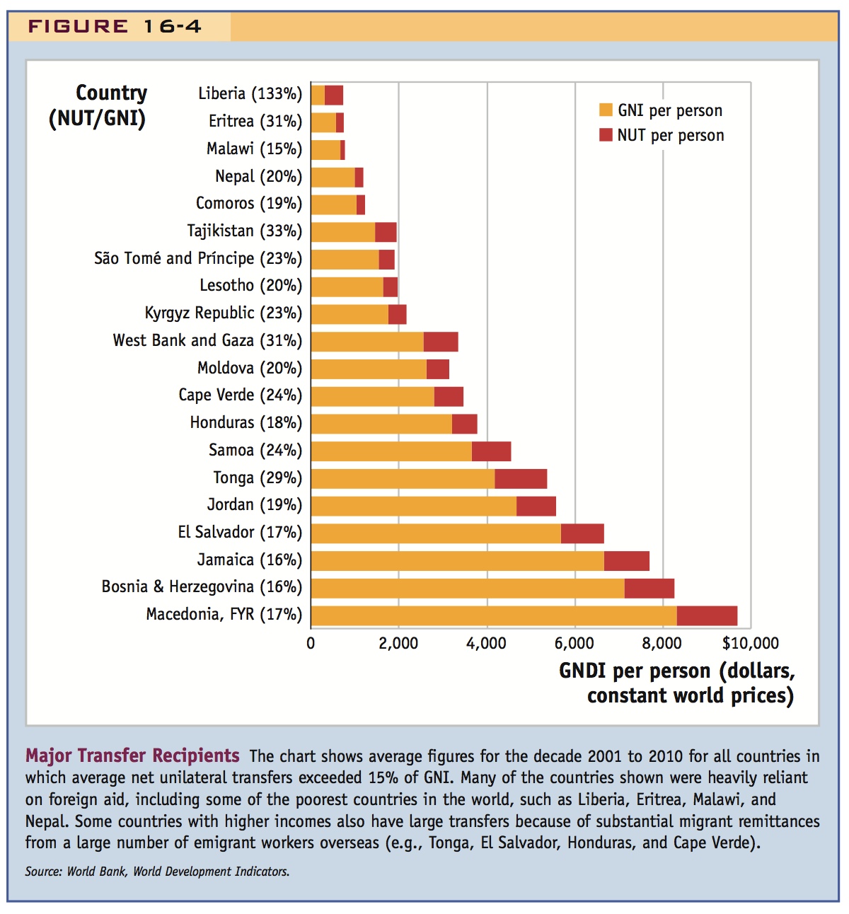
If a country receives transfers worth UTIN and gives transfers worth UTOUT, then its net unilateral transfers, NUT, are NUT = UTIN − UTOUT. Because this is a net amount, it may be positive or negative. In the year 2012, the United States had net unilateral transfers of $157 billion to the rest of the world. In general, net unilateral transfers play a small role in the income and product accounts for most high-income countries (net outgoing transfers are typically no more than 5% of GNI). But they are an important part of the gross national disposable income (GNDI) for many low-income countries that receive a great deal of foreign aid or migrant remittances, as seen in Figure 16-4.
Measuring national generosity is highly controversial and a recurring theme of current affairs (see Headlines: Are Rich Countries “Stingy” with Foreign Aid?). You might think that net unilateral transfers are in some ways a better measure of a country’s generosity toward foreigners than official development assistance, which is but one component. For example, looking at the year 2000, a USAID report, Foreign Aid in the National Interest, claimed that while U.S. ODA was only $9.9 billion, other U.S. government assistance (such as contributions to global security and humanitarian assistance) amounted to $12.7 billion, and assistance from private U.S. citizens totaled $33.6 billion—for total foreign assistance equal to $56.2 billion, more than five times the level of ODA.
To include the impact of aid and all other transfers in the overall calculation of a country’s income resources, we add net unilateral transfers to gross national income. Using the definition of GNI in Equation (5-2), we obtain a full measure of national income in an open economy, known as gross national disposable income (GNDI), henceforth denoted Y:
168
In general, economists and policy makers prefer to use GNDI to measure national income. Why? GDP is not a true measure of income because, unlike GNI, it does not include net factor income from abroad. GNI is not a perfect measure either because it leaves out international transfers. GNDI is a preferred measure because it most closely corresponds to the resources available to the nation’s households, and national welfare depends most closely on this accounting measure.
What the National Economic Aggregates Tell Us
We have explained all the international flows shown in Figure 16-2 and have developed three key equations that link the important national economic aggregates in an open economy:
- To get from GNE to GDP, we add TB (Equation 5-1).
- To get from GDP to GNI, we add NFIA (Equation 5-2).
- To get from GNI to GDNI, we add NUT (Equation 5-3).
169
Are Rich Countries “Stingy” with Foreign Aid?
The Asian tsunami on December 26, 2004, was one of worst natural disasters of modern times. Hundreds of thousands of people were killed and billions of dollars of damage was done. Some aftershocks were felt in international politics. Jan Egeland, United Nations Under-Secretary-General for Humanitarian Affairs and Emergency Relief Coordinator, declared, “It is beyond me why we are so stingy.” His comments rocked the boat in many rich countries, especially in the United States where official aid fell short of the UN goal of 0.7% of GNI. However, the United States gives in other ways, making judgments about stinginess far from straightforward.
Is the United States stingy when it comes to foreign aid?…The answer depends on how you measure….
In terms of traditional foreign aid, the United States gave $16.25 billion in 2003, as measured by the Organization of Economic Cooperation and Development (OECD), the club of the world’s rich industrial nations. That was almost double the aid by the next biggest net spender, Japan ($8.8 billion). Other big donors were France ($7.2 billion) and Germany ($6.8 billion).
But critics point out that the United States is much bigger than those individual nations. As a group, member nations of the European Union have a bit larger population than the United States and give a great deal more money in foreign aid—$49.2 billion altogether in 2003.

In relation to affluence, the United States lies at the bottom of the list of rich donor nations. It gave 0.15% of gross national income to official development assistance in 2003. By this measure, Norway at 0.92% was the most generous, with Denmark next at 0.84%.
Bring those numbers down to an everyday level and the average American gave 13 cents a day in government aid, according to David Roodman, a researcher at the Center for Global Development (CGD) in Washington. Throw in another nickel a day from private giving. That private giving is high by international standards, yet not enough to close the gap with Norway, whose citizens average $1.02 per day in government aid and 24 cents per day in private aid….
[Also], the United States has a huge defense budget, some of which benefits developing countries. Making a judgment call, the CGD includes the cost of UN peacekeeping activities and other military assistance approved by a multilateral institution, such as NATO. So the United States gets credit for its spending in Kosovo, Australia for its intervention in East Timor, and Britain for military money spent to bring more stability to Sierra Leone….
“Not to belittle what we are doing, we shouldn’t get too self-congratulatory,” says Frederick Barton, an economist at the Center for Strategic and International Studies in Washington.
Source: Republished with permission of Christian Science Monitor, from “Foreign Aid: Is the U.S. Stingy?” Christian Science Monitor/MSN Money, January 6, 2005; permission conveyed through Copyright Clearance Center, Inc.
To go one step further, we can group the three cross-border terms into an umbrella term that is called the current account CA:
170
It is important to understand the intuition for this expression. On the left is our full income measure, GNDI. The first term on the right is GNE, which measures payments by home entities. The other terms on the right, combined into CA, measure all net payments to the home country arising from the full range of international transactions in goods, services, and income.
Remember that in a closed economy, there are no international transactions so TB and NFIA and NUT (and hence CA) are all zero. Therefore, in a closed economy, the four main aggregates GNDI, GNI, GDP, and GNE are exactly equal. In an open economy, however, each of these four aggregates can differ from the others.
Understanding the Data for the National Economic Aggregates
Now that we’ve learned how a nation’s principal economic aggregates are affected by international transactions in theory, let’s see how this works in practice. In this section, we take a look at some data from the real world to see how they are recorded and presented in official statistics.
Table 16-1 shows data for the United States in 2012 reported by the Bureau of Economic Analysis in the official national income and product accounts.
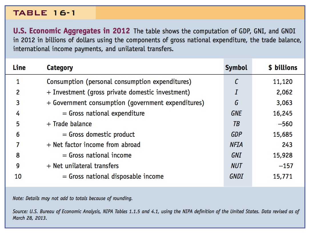
Lines 1 to 3 of the table show the components of gross national expenditure GNE. Personal consumption expenditures C were $11,120 billion, gross private domestic investment I was $2,062 billion, and government consumption G was $3,063 billion. Summing up, GNE was $16,245 billion (line 4).
Line 5 shows the trade balance TB, the net export of goods and services, which was −$560 billion. (Net exports are negative because the United States imported more goods and services than it exported.) Adding this to GNE gives gross domestic product GDP of $15,685 billion (line 6). Next we account for net factor income from abroad NFIA, +$243 billion (line 7). Adding this to GDP gives gross national income GNI of $15,928 billion (line 8).
171
Finally, to get to the bottom line, we account for the fact that the United States received net unilateral transfers from the rest of the world of −$157 billion (i.e., the United States makes net transfers to the rest of the world of $157 billion) on line 9. Adding these negative transfers to GNI results in a gross national disposable income GNDI of $15,771 billion on line 10.
Some Recent Trends Figures 5-5 and 5-6 show recent trends in various components of U.S. national income. Examining these breakdowns gives us a sense of the relative economic significance of each component.
Talk about both figures 16-5 & 16-6 in class.
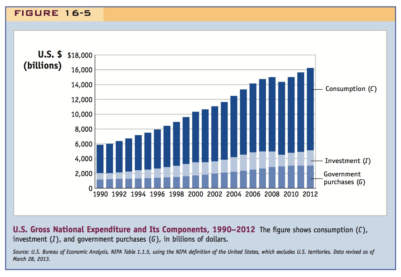
In Figure 16-5, GNE is shown as the sum of consumption C, investment I, and government consumption G. Consumption accounts for about 70% of GNE, while government consumption G accounts for about 15%. Both of these components are relatively stable. Investment accounts for the rest of GNE (about 15%), but investment tends to fluctuate more than C and G (e.g., it fell steeply after the Great Recession in 2008–2010). Over the period shown, GNE grew from $6,000 billion to around $16,000 billion in current dollars.
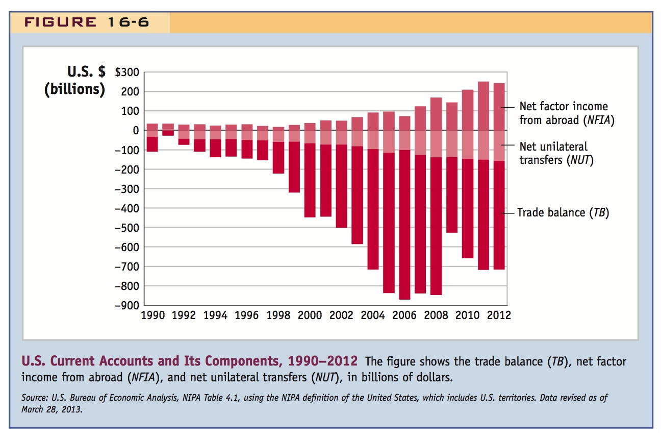
Figure 16-6 shows the trade balance (TB), net factor income from abroad (NFIA), and net unilateral transfers (NUT), which constitute the current account (CA). In the United States, the trade balance is the dominant component in the current account. For the entire period shown, the trade balance has been in deficit and has grown larger over time. From 2004 to 2008, the trade balance was close to −$800 billion, but it fell during the recession as global trade declined and then rebounded somewhat.
172
Net unilateral transfers, a smaller figure, have been between −$100 and −$150 billion in recent years.6 Net factor income from abroad was positive in all years shown, and has recently been in the range of $100 to $250 billion.
What the Current Account Tells Us
Because it tells us, in effect, whether a nation is spending more or less than its income, the current account plays a central role in economic debates. In particular, it is important to remember that Equation (5-4) can be concisely written as

This equation is the open-economy national income identity. It tells us that the current account represents the difference between national income Y (or GNDI) and gross national expenditure GNE (or C + I + G). Hence,
GNDI is greater than GNE if and only if CA is positive, or in surplus.
This can't be emphasized enough. In an ideal world people wouldn't be allowed to vote if they didn't understand this. Note that it should be an identity, not an equality though.
GNDI is less than GNE if and only if CA is negative, or in deficit.
Subtracting C + G from both sides of the last identity, we can see that the current account is also the difference between national saving (S = Y − C − G) and investment:

173
where national saving is defined as income minus consumption minus government consumption. This equation is called the current account identity even though it is just a rearrangement of the national income identity. Thus,
S is greater than I if and only if CA is positive, or in surplus.
A very nice example at this point is the historical evolution of the U.S. CA. Ask the students if the U.S. ran CA surpluses or deficits in the 19th century. Most will say surpluses. But then explain why S was low and I was high, so we had CA deficits--matched by CA surpluses in Europe.
Ask students if a CA surplus is desirable or not. What are we borrowing for?
S is less than I if and only if CA is negative, or in deficit.
These last two equations give us two ways of interpreting the current account, and tell us something important about a nation’s economic condition. A current account deficit measures how much a country spends in excess of its income or—equivalently—how it saves too little relative to its investment needs. (A currrent account surplus means the opposite.) We can now understand the widespread use of the current account deficit in the media as a measure of how a country is “spending more than it earns” or “saving too little” or “living beyond its means.”
Reports trends in S and I in industrialized economies since 1970; decomposes national saving S into private saving Sp and government saving Sg to express the fundamental identity as CA = Sp + Sg – I, and uses it to explain changes in CAs.
Global Imbalances
We can apply what we have learned to study some remarkable features of financial globalization in recent years, including the explosion in global imbalances: the widely discussed current account surpluses and deficits that have been of great concern to policy makers.
Figure 16-7 shows trends since 1970 in saving, investment, and the current account for four groups of industrial countries. All flows are expressed as ratios relative to each region’s GDP. Some trends stand out. First, in all four cases, saving and investment have been on a marked downward trend for the past 30 years. From its peak, the ratio of saving to GDP fell by about 8 percentage points in the United States, about 15 percentage points in Japan, and about 6 percentage points in the Eurozone and other countries. Investment ratios typically followed a downward path in all regions, too. In Japan, this decline was steeper than the decline in savings, but in the United States, there was hardly any decline in investment.
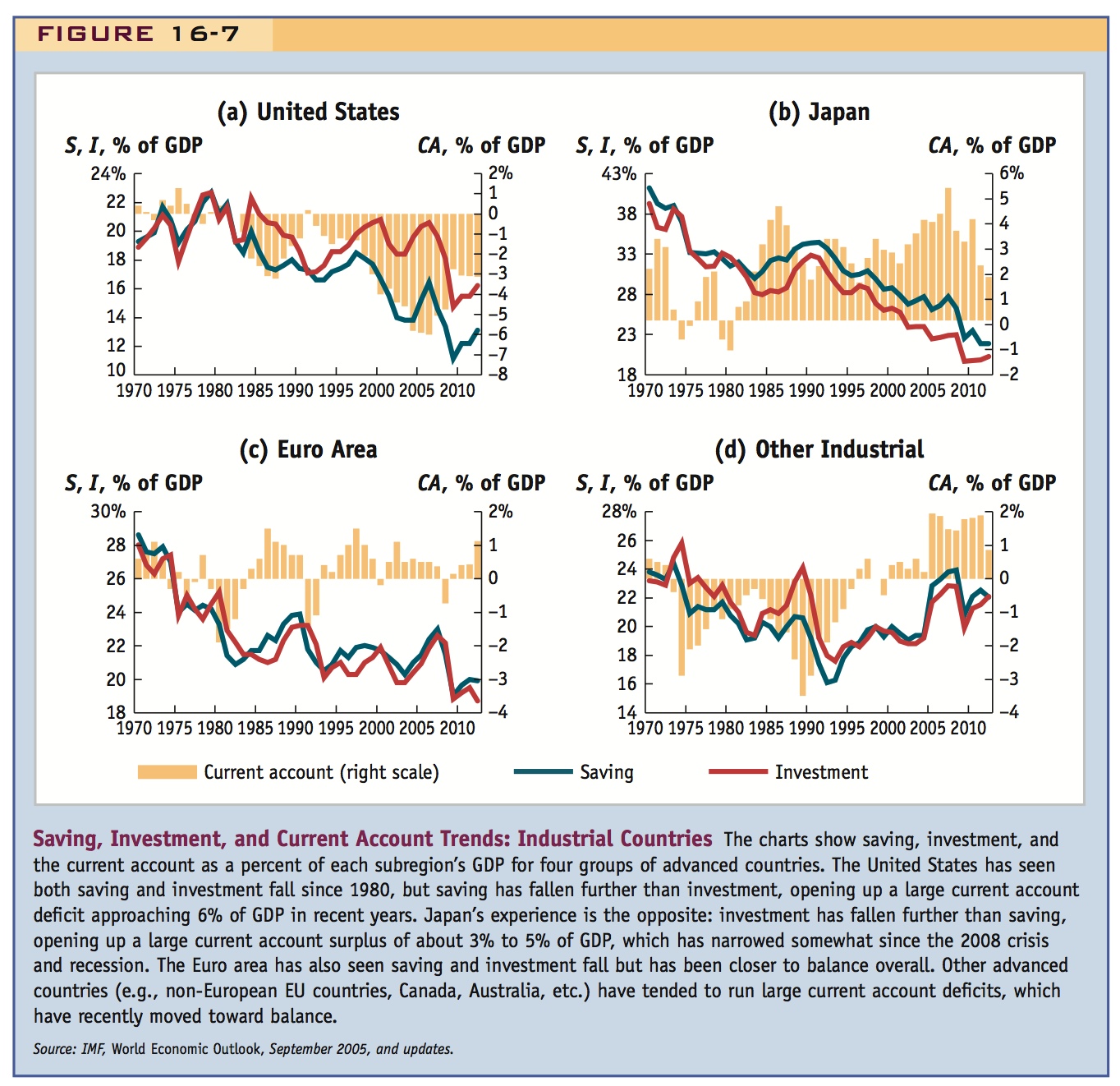
These trends reflect the recent history of the industrialized countries. The U.S. economy grew rapidly after 1990 and the Japanese economy grew very slowly, with other countries in between. The fast-growing U.S. economy generated high investment demand, while in slumping Japan investment collapsed; other regions maintained middling levels of growth and investment. Decreased saving in all the countries reflects the demographic shift toward aging populations. That is, higher and higher percentages of these nations’ populations are retired, are no longer earning income, and are living on funds they saved in the past.
The current account identity tells us that CA equals S minus I. Thus, investment and saving trends have a predictable impact on the current accounts of industrial countries. Because saving fell more than investment in the United States, the current account moved sharply into deficit, a trend that was only briefly slowed in the early 1990s. By 2003–05 the U.S. current account was at a record deficit level close to −6% of U.S. GDP, only to fall later in the Great Recession. In Japan, saving fell less than investment, so the opposite happened: a very big current account surplus opened up in the 1980s and 1990s, which closed recently. In the euro area and other industrial regions, the difference between saving and investment has been fairly steady, so their current accounts have been closer to balance.
174
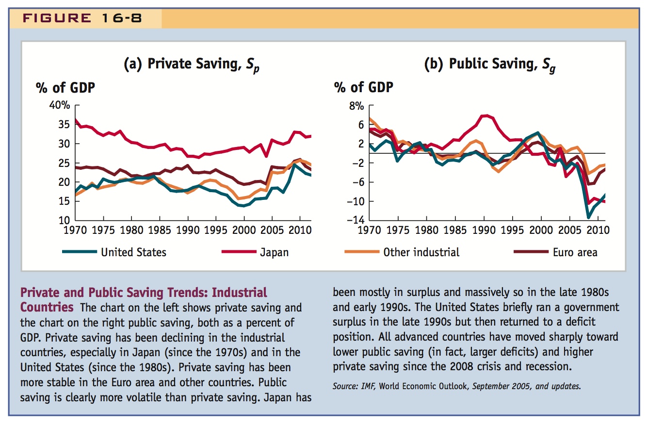
To uncover the sources of the trends in total saving, Figure 16-8 examines two of its components, public and private saving. We define private saving as the part of after-tax private sector disposable income that is not devoted to private consumption C. After-tax private sector disposable income, in turn, is national income Y minus the net taxes T paid by households to the government. Hence, private saving Sp is

Private saving can be a positive number, but if the private sector consumption exceeds after-tax disposable income, then private saving is negative. (Here, the private sector includes households and private firms, which are ultimately owned by households.)
175
Similarly, we define government saving or public saving as the difference between tax revenue T received by the government and government purchases G.7 Hence, public saving Sg equals

Government saving is positive when tax revenue exceeds government consumption (T > G) and the government runs a budget surplus. If the government runs a budget deficit, however, government consumption exceeds tax revenue (G > T), and public saving is negative.
If we add these last two equations, we see that private saving plus government saving equals total national saving

In this last equation, taxes cancel out and do not affect saving in the aggregate because they are a transfer from the private sector to the public sector.
One striking feature of the charts in Figure 16-8 is the smooth path of private saving compared with the volatile path of public saving. Public saving is government tax revenue minus spending, and it fluctuates greatly as economic conditions change. The most noticeable feature is the very large public surpluses run up in Japan in the boom of the 1980s and early 1990s which then disappeared during the long slump in the mid- to late 1990s and early 2000s. In other cases, surpluses in the 1970s soon gave way to deficits in the 1980s, and despite occasional improvements in the fiscal balance (as in the late 1990s), deficits have been the norm in the public sector. The United States witnessed a particularly sharp move from surplus to deficit after the year 2000. All regions saw private saving rise and public saving decline after the 2008 crisis and up to 2012.
176
Do government deficits cause current account deficits? Sometimes they go together: in the early 2000s, the U.S. government went into deficit when it was fighting two wars (Afghanistan and Iraq) and implemented tax cuts. At the same time there was a large increase in the current account deficit as seen in Figure 16-7. Sometimes, however, the “twin deficits” do not occur at the same time; they are not inextricably linked, as is sometimes believed. Why?
We can use the equation just given and the current account identity to write

Now, suppose the government lowers your taxes by $100 this year and borrows to finance the resulting deficit but also says you will be taxed by an extra $100 plus interest next year to pay off the debt. The theory of Ricardian equivalence asserts that you and other households will save the tax cut to pay next year’s tax increase, so that any fall in public saving will be fully offset by a rise in private saving. In this situation, the current account—as seen in Equation (5-10)—would be unchanged. However, empirical studies do not support this theory: private saving does not fully offset government saving in practice.8
How large is the effect of a government deficit on the current account deficit? Research suggests that a change of 1% of GDP in the government deficit (or surplus) coincides with a 0.2% to 0.4% of GDP change in the current account deficit (or surplus), a result consistent with a partial Ricardian offset.
A second reason why the current account might move independently of saving (public or private) is that during the same period there may be a change in the level of investment in the last equation. A comparison of Figures 5-7 and 5-8 shows this effect at work. For example, we can see from Figure 16-7 that the large U.S. current account deficits of the early to mid-1990s were driven by an investment boom, even though total saving rose slightly, driven by an increase in public saving seen in Figure 16-8. Here there was no correlation between government deficit (falling) and current account deficit (rising). Shifts after the 2008 recession illustrate multiple factors at work: U.S. investment collapsed and private saving rose as recession fears increased. The combined effects of lower investment and higher private saving more than offset the decline in public saving and so overall the current account deficit started to decline.
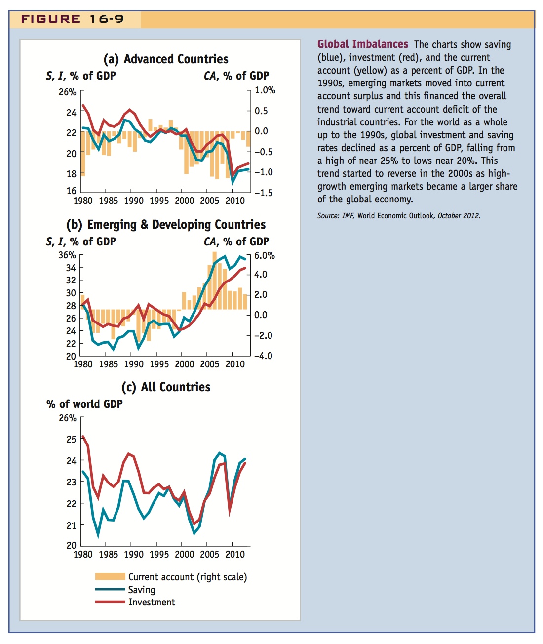
Finally, Figure 16-9 shows global trends in saving, investment, and the current account for advanced countries, emerging and developing economies, and the world economy since 1980. Because the U.S. economy accounts for a large part of the world economy, in aggregate, the industrial countries have shifted into current account deficit over this period, a trend that has been offset by a shift toward current account surplus in the developing countries. The industrialized countries all followed a trend of declining investment and saving ratios, but the developing countries saw the opposite trend: rising investment and saving ratios. For the developing countries, however, the saving increase was larger than the investment increase, allowing a current account surplus to open up. Overall, the industrial country trend of lower saving and investment drove the world trend of lower saving and investment in the 1980s and 1990s. But since the 2000s, the rising share of high-saving emerging and developing countries in the world economy has caused the world trends to reverse. Saving and investment have been on the rise in recent years, but the effects have been felt very unevenly across the globe, leading to the imbalances we have studied.
I'd recommend doing all this back around Equation 16-6.
Spend some time talking about the twin deficit hypothesis, as well as changes in the U.S. CA over the last few decades.
Talk through this in class.
177
178