1 The Limits on How Much a Country Can Borrow: The Long-Run Budget Constraint
International financial markets allow countries to borrow and lend, but there are limits to how much a country can borrow or will lend. Saving and investment allocate resources over time, so we need a dynamic approach to the economy—the intertemporal approach of macroeconomics. In the last chapter we saw how the CA affects external wealth. In this section we use external wealth to derive the long-run budget constraint (LRBC) of the economy, which forces the economy to live within its means. To develop some intuition for this, suppose you borrow some money. Consider two cases: (1) You service the debt, paying your interest each period, but not the principal, so your wealth remains constant; (2) You don’t service the debt, but just roll over the principal plus interest each year. Case (2) is called a Ponzi scheme, and is unsustainable.
1. How the Long-Run Budget Constraint Is Determined
Assumptions: (1) flexible prices; (2) the country is small in both goods and bond markets; (3) an exogenous real world interest rate that applies to both assets and liabilities, so that (4) the return to wealth in each period is r*W = r*(A - L); (5) there are no transfers.
a. Calculating the Change in Wealth in Each Period: Ignoring capital gains, wealth grows if there is a trade surplus and if there is net factor income: ΔWN = WN-WN-1 = TBN + r* WN-1.
b. Calculating Future Wealth Levels: Alternatively, WN = TBN + (1 + r* ) WN-1.
2. The Budget Constraint in a Two-Period Example
Country has inherited wealth of W1 = 0 and must pay off its debts or collect its loans in period 1, so that W1 = 0. In period 0, W0 = TB0+ (1 + r* ) W-1. Then in period 1, W1 = TB1 + (1 + r*) TB0 + (1 + r*)2 W-1. But since W1 = 0, -(1 + r*)2 W-1 = TB1+ (1 + r*) TB0. A creditor with positive initial wealth can afford to run deficits in the future.
a. Present Value Form: Alternatively, -(1 + r*) W-1 = TB0 + TB1⁄((1 + r*). The current value of wealth from last period must equal the present value (PV) of future trade balances.
b. A Two-Period Example: A numerical example of a country that starts out in debt. To pay off its debt in period 1, it must run a surplus in at least one of the two periods, so that their present value is positive.
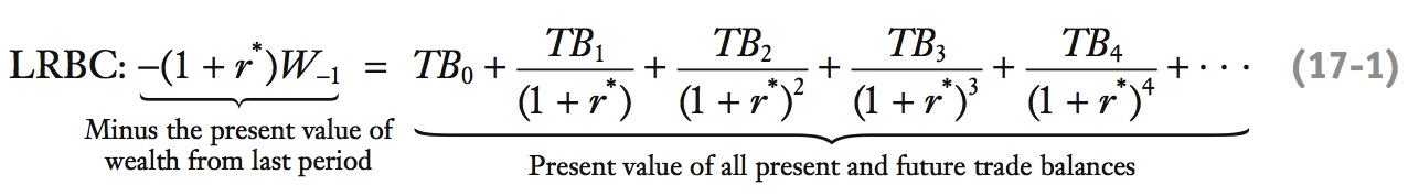
c. Extending the Theory to the Long Run: The long-run budget constraint (LRBC) generalizes this to a multi-period setting. The current value of wealth from last period must equal the PV of future trade balances:  Implication: A debtor country must run future trade balances that are positive in present value terms, while a creditor country must run trade balances that are negative in present value terms.
3. A Long-Run Example: The Perpetual Loan
The country pays a constant amount X to its creditors in each period. Use infinite geometric series to show that the present value of the payment is then X/r*. We will use this in applications.
4. Implications of the LRBC for Gross National Expenditure and Gross Domestic Product
The LRBC implies that  The present value of an economy’s resources must equal the present value of its expenditures.
5. Summary
In a closed economy, the “TB” must always be balanced. In an open economy, TBs need only be balanced in a present-value sense. Therefore an open economy should be better able to achieve a desired pattern of expenditures than a closed economy.
Our introductory examples show how borrowing can help countries (like households) better cope with shocks. But, also like households, there is a limit to how much a country can borrow (or, how much lenders will lend). Understanding the constraints on how countries might borrow and lend to each other is our critical first task in this chapter. With this understanding we can then examine how financial globalization shapes the economic choices available to a country as economic conditions change over time. The ability to borrow in times of need and lend in times of prosperity has profound effects on a country’s well-being.
This will be quite new to most students, so emphasize that nowadays all macros are dynamic.
When we study an economy as it evolves over time, we are taking a dynamic approach to macroeconomics—rather than a static approach by looking at the state of the economy at one specific time. The dynamic approach is also known as the intertemporal approach to macroeconomics. One key to this approach is that we must keep track of how a country is managing its wealth and whether it is doing so in a way that is within its means, that is, sustainable in the long run. The intertemporal approach makes use of the key lessons from the end of the last chapter, which taught us how to account for the change in a nation’s external wealth from one period to the next.
In this section, we use changes in an open economy’s external wealth to derive the key constraint that limits its borrowing in the long run: the long-run budget constraint (LRBC). The LRBC tells us precisely how and why a country must, in the long run, “live within its means.” A country’s ability to adjust its external wealth through borrowing and lending provides a buffer against economic shocks, but the LRBC places limits on the use of this buffer.
To develop some intuition, let’s look at a simple household analogy. This year (year 0) you borrow $100,000 from the bank at an interest rate of 10% annually. You have no other wealth and inflation is zero. Once you borrow the $100,000, consider two possible different ways in which you can deal with your debt each year.
Case 1 A debt that is serviced. Every year you pay the 10% interest due on the principal amount of the loan, $10,000, but you never pay any principal. At the end of each year, the bank renews the loan (a rollover), and your wealth remains constant at −$100,000.
Case 1 A debt that is not serviced. You pay neither interest nor principal but ask the bank to roll over the principal plus the interest due on it each year. In year 1, the overdue interest is $10,000, and your debt grows by 10% to $110,000. In year 2, the overdue interest is 10% of $110,000, or $11,000, and your debt grows by 10% again to $121,000. Assuming this process goes on and on, your level of debt grows by 10% every year.
Ponzi schemes always elicit class discussion.
Case 2 is not sustainable. If the bank allows it, your debt level will explode to infinity as it grows by 10% every year forever. This case, sometimes called a rollover scheme, a pyramid scheme, or a Ponzi game,1 illustrates the limits or constraints on the use of borrowing, which implies negative external wealth. In the long run, lenders will simply not allow the debt to grow beyond a certain point. Debts must be paid off eventually. This requirement is the essence of the long-run budget constraint.
How the Long-Run Budget Constraint Is Determined
As is usual when building an economic model, we start with a basic model that makes a number of simplifying assumptions, but yields lessons that can be extended to more complex cases. Here are the assumptions we make about various conditions that affect our model:
- Prices are perfectly flexible. Under this assumption, all analysis in this chapter can be conducted in terms of real variables, and all monetary aspects of the economy can be ignored. (To adjust for inflation and convert to real terms, we could divide all nominal quantities by an index of prices.)
- The country is a small open economy. The country trades goods and services with the rest of the world through exports and imports and can lend or borrow overseas, but only by issuing or buying debt (bonds). Because it is small, the country cannot influence prices in world markets for goods and services.
- All debt carries a real interest rate r*, the world real interest rate, which we assume to be constant. Because the country is small, it takes the world real interest rate as given, and we assume it can lend or borrow an unlimited amount at this interest rate.
- The country pays a real interest rate r* on its start-of-period debt liabilities L and is paid the same interest rate r* on its start-of-period debt assets A. In any period, the country earns net interest income payments equal to r*A minus r*L or, more simply, r*W, where W is external wealth (A − L) at the start of the period. External wealth may vary over time.
- There are no unilateral transfers (NUT = 0), no capital transfers (KA = 0), and no capital gains on external wealth. Under these assumptions, there are only two nonzero items in the current account: the trade balance TB and net factor income from abroad, r*W. If r*W is positive, the country is earning interest and is a lender/creditor with positive external wealth. If r*W is negative, the country is paying interest and is a borrower/debtor with negative external wealth.
203
Calculating the Change in Wealth Each Period In the previous balance of payments chapter, we saw that the change in external wealth equals the sum of three terms: the current account, the capital account, and capital gains on external wealth. In the special case we are studying, our assumptions tell us that the last two terms are zero, and that the current account equals the sum of just two terms: the trade balance TB plus any net interest payments r*W at the world interest rate on the external wealth held at the end of the last period.
In passing, point out that this formalizes the intuition developed in the last chapter, that CS surpluses will cause wealth to grow.
Mathematically, we can write the change in external wealth from end of year N − 1 to end of year N as follows (where subscripts denote periods, here years):
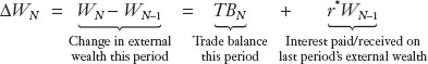
In this simplified world, external wealth can change for only two reasons: surpluses or deficits on the trade balance in the current period, or surpluses and deficits on net factor income arising from interest received or paid.
Calculating Future Wealth Levels Now that we have a formula for wealth changes, and assuming we know the initial level of wealth in year N − 1, we can compute the level of wealth at any time in the future by repeated application of the formula.
To find wealth at the end of year N, we rearrange the preceding equation:
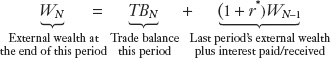
This equation presents an important and intuitive result: it shows that wealth at the end of a period is the sum of two terms. The trade balance this period captures the addition to wealth from net exports (exports minus imports). Wealth at the end of last period times (1 + r*) captures the wealth from last period plus the interest earned on that wealth. The examples in the following sections will help us understand the changes in a country’s external wealth and the role that the trade balance plays here.
The Budget Constraint in a Two-Period Example
Define it as W0.
We first put these ideas to work in a simplified two-period example. Suppose we start in year 0, so N = 0. Suppose further that a country has some initial external wealth from year −1 (an inheritance from the past), and can borrow or lend in the present period (year 0). We also impose the following limit: by the end of year 1, the country must pay off what it has borrowed from other countries and must call in all loans it has made to other countries. That is, the country must end year 1 with zero external wealth.
As we saw in the formula given earlier, W0 = (1 + r*) W−1 + TB0. Wealth at the end of year 0 depends on two things. At the end of year 0, the country carries over from the last period (year −1) its initial wealth level, plus any interest accumulated on it. In addition, if the country runs a trade deficit it has to run its external wealth down by adding liabilities (borrowing) or cashing in external assets (dissaving); conversely, if the country runs a trade surplus, it lends that amount to the rest of the world.
That’s the end of year 0. But next, where do things stand at the end of year 1? We assume the country must have zero external wealth when the world ends at the end of year 1. Applying the preceding formula to year 1, we know that W1 = 0 = (1 + r*) W0 + TB1. We can then substitute W0 = (1 + r*) W−1 + TB0 into this formula to find that
204
W1 = 0 = (1 + r*)2W−1 + (1 + r*)TB0 + TB1
This equation shows that two years later at the end of year 1 the country has accumulated wealth equal to the trade balance in years 0 and 1 (TB0 + TB1); plus one year of interest earned (or paid) on the year 0 trade balance (r*TB0); plus the two years of interest and principal earned (or paid) on its initial wealth (1 + r*)2W−1.
Because we have stated that the final wealth level W1 must be zero, the right-hand side of the last equation must be zero, too. For that to be the case, the trade balances in year 0 (TB0) and in year 1 (TB1) (plus any accumulated interest) must be equal and opposite to initial wealth (W−1) (plus any accumulated interest):
−(1 + r*)2W−1 = (1 + r*)TB0 + TB1
This equation is the two-period budget constraint. It tells us that a creditor country with positive initial wealth (left-hand-side negative) can afford to run trade deficits “on average” in future; conversely, a debtor country (left-hand-side positive) is required to run trade surpluses “on average” in future.
Beware: Some of the students won't really understand present values. Be prepared to talk about the time value of money and discounting. A neat example that gets their interest is of winning a lottery for $1,000,000: If it is paid out in five installments, what is it really worth today? Then change interest rates to see what happens to the present value.
Present Value Form By dividing the previous equation by (1 + r*), we find a more intuitive expression for the two-period budget constraint:
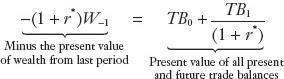
Every element in this statement of the two-period budget constraint represents a quantity expressed in so-called present value terms.
By definition, the present value of X in period N is the amount that would have to be set aside now, so that, with accumulated interest, X is available N periods from now. If the interest rate is r*, then the present value of X is X/(1 + r*)N. For example, if you are told that you will receive $121 at the end of year 2 and the interest rate is 10%, then the present value of that $121 now, in year 0, is $100 because $100 × 1.1 (adding interest earned in year 1) × 1.1 (adding interest earned in year 2) = $121.
A Two-Period Example Let’s put some numbers into the last equation. Suppose a country starts in debt, with a wealth level of −$100 million at the end of year −1: W−1 = −$100 million. Question: at a real interest rate of 10%, how can the country satisfy the two-period budget constraint that it must have zero external wealth at the end of year 1? Answer: to pay off the $110 million (initial debt plus the interest accruing on this debt during period 0) on the left-hand side, the country must ensure that the present value of future trade balances TB1 is +$110 million on the right-hand side.
A starker example would be to assume initial wealth is zero. Point out that a trade deficit in the first period would have to financed by a trade surplus in the second period.
The country has many ways to do this.
- It could pay off its debt at the end of period 0 by running a trade surplus of $110 million in period 0 and then have balanced trade in period 1.
- It could wait to pay off the debt until the end of period 1 by having balanced trade in period 0 and then running a trade surplus of $121 million in period 1.
- It could pay off the debt and its accumulated interest through any other combination of trade balances in periods 0 and 1, as long as external wealth at the end of period 1 is zero and the budget constraint is satisfied.
205
Extending the Theory to the Long Run By extending the two-period model to N periods, and allowing N to run to infinity, we can transform the two-period budget constraint into the long-run budget constraint (LRBC). Repeating the two-period logic N times, external wealth after N periods is initial wealth and accumulated interest on that wealth (whether positive or negative) plus all intervening trade balances and accumulated interest on those positive or negative trade balances. If external wealth is to be zero at the end of N periods, then the sum of the present values of N present and future trade balances must equal minus the present value of external wealth. If N runs to infinity, we get an infinite sum and arrive at the equation of the LRBC:2
Now generalize this intuition for many periods.
This expression for the LRBC says that a debtor country must have future trade balances that are positive in present value terms so that they offset the country’s initially negative wealth. Conversely, a creditor country must have future trade balances that are negative in present value terms so that they offset the country’s initially positive wealth. The LRBC plays an important role in our analysis of how countries can lend or borrow because it imposes a condition that rules out choices that would lead to exploding positive or negative external wealth.
A Long-Run Example: The Perpetual Loan
The following example helps us understand the long-run budget constraint and we can apply it to various cases that we visit in the rest of the chapter. It shows us how countries that take out an initial loan must make payments to service that loan in the future.
Suppose that today is year 0 and a country is to pay (e.g., to its creditors) a constant amount X every year starting next year, year 1. What is the present value (PV) of that sequence of payments (X)?
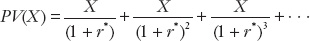
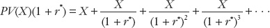
This expression for PV(X) is an infinite sum. If we multiply this equation by (1 + r*), we obtain
206
To find a simple expression for PV(X), we subtract the first equation from the second, cancel out all of the terms on the right except X, then rearrange the remaining equation r*PV(X) = X to arrive at:

Maybe use this to derive the price of a consol bond, or of a stock that pays constant dividends in perpetuity.
This formula helps us compute PV(X) for any stream of constant payments, something we often need to do to verify the long-run budget constraint.
Alternatively, point out that this is an infinite geometric series and use that formula. Students are likely to have encountered this in the money multiplier, or the Keynesian multiplier, in a finance class, or even in a stats class.
For example, if the constant payment is X = 100 and the interest rate is 5% (r* = 0.05), Equation (6-2) says that the present value of a stream of payments of 100 starting in year 1 is 100/0.05 = 2,000:

This example, which we will often revisit later in this chapter, shows the stream of interest payments on a perpetual loan (i.e., an interest-only loan or, equivalently, a sequence of loans for which only the principal is refinanced or rolled over every year). If the amount loaned by the creditor is $2,000 in year 0, and this principal amount is outstanding forever, then the interest that must be paid each year to service the debt is 5% of $2,000, or $100. Under these conditions, wherein the loan payments are always fully serviced, the present value of the future interest payments equals the value of the amount loaned in year 0 and the LRBC is satisfied.
Implications of the LRBC for Gross National Expenditure and Gross Domestic Product
In economics, a budget constraint always tells us something about the limits to expenditure, whether for a person, firm, or government. The LRBC is no different—it tells us that in the long run, a country’s national expenditure (GNE) is limited by how much it produces (GDP).
A fundamental result. Emphasize it by writing down the two period version, and depicting the two-period budget constraint, a la Fisher.
To see why this is true, recall from the previous chapter that the trade balance is the difference between gross domestic product and gross national expenditure, TB = GDP − GNE. If we insert this expression into the LRBC equation (6-1) and collect terms, we see that
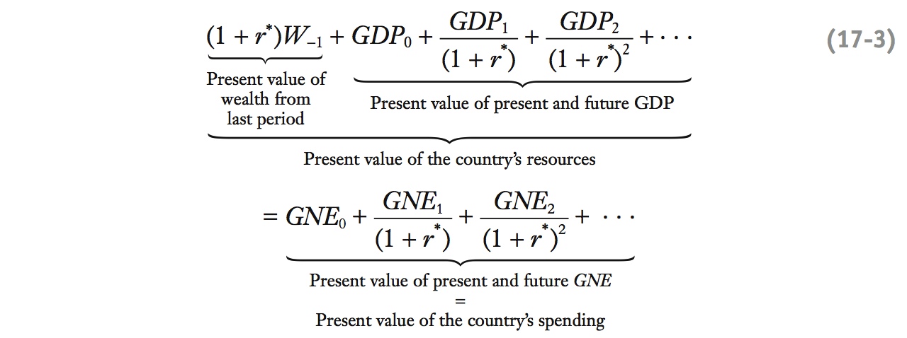
The left side of this equation is the present value of the country’s resources in the long run: the present value of any inherited wealth plus the present value of present and future product as measured by GDP. The right side is the present value of all present and future spending (C + I + G) as measured by GNE.
207
We have arrived at the following, very important result: the long-run budget constraint says that in the long run, in present value terms, a country’s expenditures (GNE) must equal its production (GDP) plus any initial wealth. The LRBC states that an economy must live within its means in the long run.
Summary
Drive this home: it gives a precise meaning to "living within our means," but also suggests the benefits of not being forced to live within one's means year by year.
The key lesson of our intertemporal model is that a closed economy is subject to a tighter budget constraint than an open economy. In a closed economy, “living within your means” requires a country to have balanced trade each and every year. In an open economy, “living within your means” requires only that a country must maintain a balance between its trade deficits and surpluses that satisfies the long-run budget constraint—they must balance only in a present value sense, rather than year by year.
This conclusion implies that an open economy should be able to do better (or no worse) than a closed economy in achieving its desired pattern of expenditure over time. This is the essence of the theoretical argument that there are gains from financial globalization.
In the next section, we examine this argument in greater detail and consider under what circumstances it is valid in the real world. First, however, we consider some situations in which the assumptions of the model might need to be modified.
We assumed that (1) the same interest rate applied to income from both assets and liabilities, and that (2) there were no capital gains. Neither assumption applies to the U.S.
a. “Exorbitant Privilege”: The U.S. is a debtor, yet earns positive net factor income. This is because, as the “world’s banker,” it gets higher interest on its assets than on its liabilities.
b. “Manna from Heaven”: The U.S. also enjoys substantial capital gains on its external wealth.
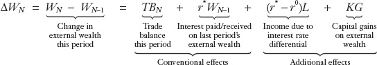
c. Summary: For the U.S. WN - WN-1 = TBN + r* WN-1 + (r* - r0 )L+ KG, where the last two terms are the differential interest income and capital gains just described.
d. Too Good to Be True? These terms allow the U.S. to offset losses in wealth caused by its trade deficits. Some say this means deficits are nothing to worry about; others say these factors are unsustainable and diminishing over time. Gros says these putative effects can be explained by measurement errors; correcting them doubles U.S. indebtedness.
If you just drew the two-period budget constraint, draw a new, kinked one for this case.
Invite discussion about why the U.S. has this exorbitant privilege.
A good place to link this discussion back to the valuation effects in the last chapter.
The Favorable Situation of the United States
Two assumptions greatly simplified our intertemporal model. We assumed that the same real rate of interest r* applied to income received on assets and income paid on liabilities, and we assumed that there were no capital gains on external wealth. However, these assumptions do not hold true for the United States.
“Exorbitant Privilege” Since the 1980s, the United States has been the world’s largest ever net debtor with W = A − L < 0. Under the model’s simplifying assumptions, negative external wealth would lead to a deficit on net factor income from abroad with r*W = r* (A − L) < 0. And yet as we saw in the last chapter, U.S. net factor income from abroad has been positive throughout this period! How can this be?
The only way a net debtor can earn positive net interest income is by receiving a higher rate of interest on its assets than it pays on its liabilities. The data show that this has been consistently true for the United States since the 1960s. The interest the United States has received on its assets has been higher by about 1.5 to 2 percentage points per year on average (with a slight downward trend) than the interest it pays on its liabilities.
To develop a framework to make sense of this finding, suppose the United States receives interest at the world real interest rate r* on its external assets but pays interest at a lower rate r0 on its liabilities. Then its net factor income from abroad is r*A − r0 L = r*W + (r* − r0)L. The final term, the interest rate difference times total liabilities, is an income bonus the United States earns as a “banker to the world”—like any other bank, it borrows low and lends high.
Understandably, the rest of the world may resent this state of affairs from time to time. In the 1960s French officials complained about the United States’ “exorbitant privilege” of being able to borrow cheaply by issuing external liabilities in the form of reserve assets (Treasury debt) while earning higher returns on U.S. external assets such as foreign equity and foreign direct investment. This conclusion is not borne out in the data, however. U.S. Bureau of Economic Analysis (BEA) data suggest that most of the interest rate difference is due not to the low interest paid on Treasury debt, but to the low interest rate on U.S. equity liabilities (i.e., low profits earned on foreign investment in the United States).3
208
“Manna from Heaven” The difference between interest earned and interest paid isn’t the only deviation from our simple model that benefits the United States. BEA statistics reveal that the country has long enjoyed positive capital gains (KG) on its external wealth. This gain, which started in the 1980s, comes from a difference of two percentage points between large capital gains on several types of external assets and smaller capital losses on external liabilities.
It is hard to pin down the source of these capital gains because the BEA data suggest that these effects are not the result of price or exchange rate effects, and they just reflect capital gains that cannot be otherwise measured. As a result, the accuracy and meaning of these measurements is controversial. Some skeptics call these capital gains “statistical manna from heaven.” Others think these gains are real and may reflect the United States acting as a kind of “venture capitalist to the world.” As with the “exorbitant privilege,” this financial gain for the United States is a loss for the rest of the world.4
Summary When we add the 2% capital gain differential to the 1.5% interest differential, we end up with a U.S. total return differential (interest plus capital gains) of about 3.5% per year on average since the 1980s. For comparison, in the same period, the total return differential was close to zero in every other G7 country.
To include the effects of the total return differential in our model, we have to incorporate the effect of the extra “bonuses” on external wealth as well as the conventional terms that reflect the trade balance and interest payments:
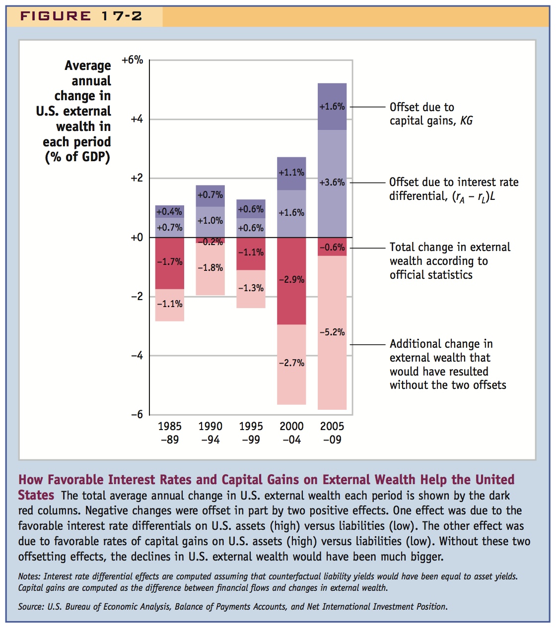
Too Good to Be True? With this equation, the implications of the final two terms become clearer for the U.S. economy. When positive, they offset wealth losses due to trade deficits. Thus, if these terms increase in value by 1% of GDP, for example, then the United States could run an additional 1% of GDP in trade deficit forever and still satisfy its LRBC.
As Figure 17-2 shows, the United States has seen these offsets increase markedly in recent years, rising from 1% of GDP in the late 1980s to an average of about 4% of GDP in the 2000s. These large offsets have led some economists to take a relaxed view of the swollen U.S. trade deficit because the offsets finance a large chunk of the country’s trade deficit—with luck, in perpetuity.5 However, we may not be able to count on these offsets forever: longer-run evidence suggests that they are not stable and may be diminishing over time.6
209
Others warn that, given the likely presence of errors in these data, we really have no idea what is going on. In 2006, economist Daniel Gros calculated that the United States had borrowed $5,500 billion over 20 years, even though its external wealth had fallen by “only” $2,800 billion. Have $2.7 trillion dollars been mislaid? Gros argued that most of this difference can be attributed to poor U.S. measurement of the assets foreigners own and investment earnings foreigners receive. Correcting these errors would make all of the additional offset terms disappear—and roughly double the estimated current level of U.S. net indebtedness to the rest of the world.7
Another good place for class discussion. Can we afford to be insouciant about our CA deficit, especially if Gros is right?
210
A nice example to use, both because it is symmetric to the U.S. case (draw the two-period budget constraint), and because it has important policy implications.
The assumptions of the basic model also often fail for poor, developing countries. First, they often have to pay a risk premium when they borrow. Second, they often face credit constraints.
The Difficult Situation of the Emerging Markets
The previous application showed that the simple intertemporal model may not work for the United States. In this section, we see that its assumptions may also not work for emerging markets and developing countries.
As in the U.S. example, the first assumption we might question is that these nations face the same real interest rate on assets and liabilities. The United States borrows low and lends high. For most poorer countries, the opposite is true. Because of country risk, investors typically expect a risk premium before they will buy any assets issued by these countries, whether government debt, private debt or equity, or foreign direct investments.
Figure 17-3 plots government credit ratings (from Standard & Poor’s) against public debt levels using historical data prior to the financial crisis of 2008 for a large sample of countries. Bond ratings are seen to be highly correlated with risk premiums. At the top of the figure are the advanced countries whose bonds were then rated AA or better. (At the time this sample was constructed, before the financial crisis, almost all the advanced countries had very high credit ratings and moderate debt levels; after the financial crisis and Great Recession, this rapidly changed as some advanced countries’ debt rapidly ballooned and their credit ratings fell: some of them even fell quite far and started to look more like emerging markets).
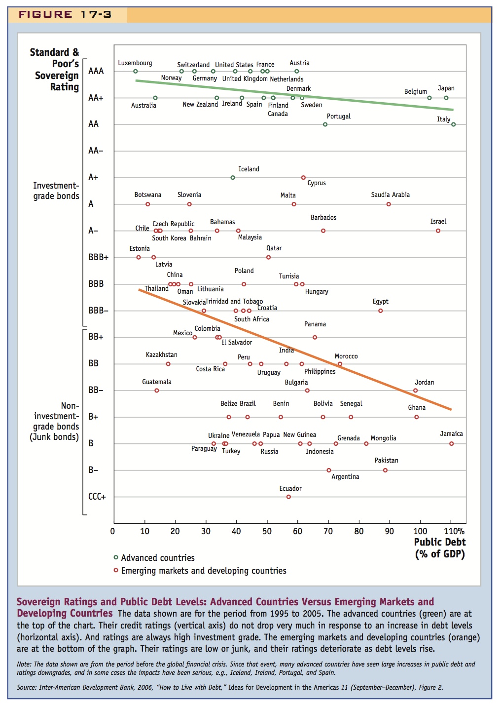
Before the financial crisis, advanced-country bonds carried very small-risk premiums because investors were confident that these countries would repay their debts. In addition, the risk premiums did not increase markedly even as these countries went further into debt. In the bottom half of the figure, we see that emerging markets and developing countries inhabited a very different world. They had worse credit ratings and correspondingly higher-risk premiums. Only about half of the government bonds issued by these countries were considered investment grade, BBB− and above; the rest were considered junk bonds. Investors demanded extra profit as compensation for the perceived risks of investing in many of these countries.
Figure 17-3 also shows that in poorer countries ratings deteriorated rapidly as debt levels rose, an effect that is not as strong in the advanced countries. This observation shows the sharp limits to borrowing for poorer countries: at some stage, the cost of borrowing becomes prohibitive, if it is possible at all.
This example brings us to the other assumption of the simple model that sometimes fails to hold in poorer countries, the assumption that the country can borrow or lend as much as it wants at the prevailing world real interest rate. On the lending side, it usually isn’t a problem to save as much as you want. On the borrowing side, however, lenders often tell borrowers that they have reached a debt limit and can borrow no more. When that happens, access to external credit ceases, and anything additional a country wants to consume or invest has to be taken out of its own domestic output.
211
212
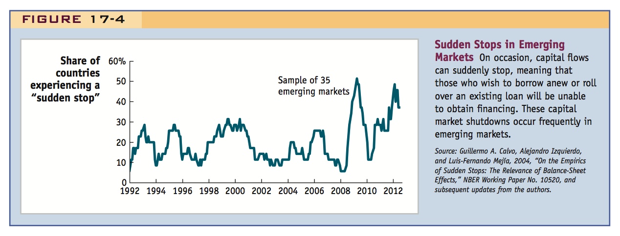
Figure 17-4 illustrates the remarkable frequency with which emerging market countries experience this kind of isolation from global capital markets. Research by economists Guillermo Calvo and Carmen Reinhart has focused attention on sudden stops in the flow of external finance, especially in emerging markets.8 In a sudden stop, a borrower country sees its financial account surplus rapidly shrink (suddenly nobody wants to buy any more of its domestic assets) and so the current account deficit also must shrink (because there is no way to finance a trade imbalance). Reaching a debt limit can be a jolting macroeconomic shock for any economy, because it requires sudden and possibly large adjustments to national expenditure and its composition. Most seriously, output may drop if domestic investment is curtailed as a result of lack of access to external credit. As the constraints arising from hitting a debt limit start to bite, the upside of financial globalization recedes, and the downside of economic instability may take its place. In later chapters, we examine why credit market disruptions happen by looking in more detail at financial problems, crises, and default.