4 Gains from Diversification of Risk
Another way financial globalization may be beneficial is by permitting diversification.
1. Diversification: A Numerical Example and Generalization
Assume two countries, A and B, and output has two states, 1 and 2. The shocks are symmetrical: If A is in a bad state B is a good state, and vice versa. All output is consumed and capital’s share is .4. The critical question is who owns the claims to capital income:
a. Home Portfolios
Case 1: Households in each country own all of their respective capital stocks. All fluctuations in output in each country are mirrored in fluctuations in consumption, but world output is the same.
b. World Portfolios
Case 2: The risk is diversified by letting households in each country own half of the other country’s capital stock. Now GNI can differ from GDP. Labor incomes still fluctuate, but capital income is smoothed. In a bad state, A receives capital income from its external assets in B; this allows A to smooth its consumption by running a TB deficit. Diversification reduces the fluctuations in consumption.
c. Generalizing
If shocks are asymmetric (perfect negative correlation) then the volatility can be eliminated by holding a diversified portfolio. If the shocks are common (perfect positive correlation) then there are no gains from diversification. More generally, there are gains from diversification as long as shocks are not perfectly correlated.
d. Limits to Diversification: Capital Versus Labor Income
Labor income is not diversifiable. However, since labor and capital income tend to move together; trading claims to capital may serve as a substitute for trading claims to labor.
In the second section of this chapter, we studied consumption smoothing using a simplified model. We used a borrowing and lending approach, we considered a small open economy, we assumed that countries owned their own output, and we treated output shocks as given. We then saw how debt can be used to smooth the impact of output shocks on consumption. However, we also discussed the finding that in practice, countries seem to be unable to eliminate the effects of output volatility. The problems seem to be especially difficult in emerging markets and developing countries. We also saw that reliance on borrowing and lending may create problems because there may be limits to borrowing, risk premiums, and sudden stops in the availability of credit.
237
Are there other ways for a country to cope with shocks to output? Yes. In this final section, we show how diversification, another facet of financial globalization, can help smooth shocks by promoting risk sharing. With diversification, countries own not only the income stream from their own capital stock, but also income streams from capital stocks located in other countries. We see how, by using financial openness to trade such rights—for example, in the form of capital equity claims like stocks and shares—countries may be able to reduce the volatility of their incomes (and hence their consumption levels) without any net lending or borrowing whatsoever.
Diversification: A Numerical Example and Generalization
In this case we are stuck with the numerical example, since expositing it more generally requires fancier tools.
To keep things simple and to permit us to focus on diversification, we assume there is no borrowing (the current account is zero at all times). To illustrate the gains from diversification, we examine the special case of a world with two countries, A and B, which are identical except that their respective outputs fluctuate asymmetrically, that is, they suffer equal and opposite shocks.
We now explore how this world economy performs in response to the output shocks. We examine the special case in which there are two possible “states of the world,” which are assumed to occur with an equal probability of 50%. In terms of output levels, state 1 is a bad state for A and a good state for B; state 2 is a good state for A and a bad state for B.
We assume that all output is consumed, and that there is no investment or government spending. As we know from the previous chapter, output is distributed to factors in the form of income. We assume output is divided 60–40 between labor income and capital income in each country. The key question for us is who owns this income: domestic residents or foreigners?
Home Portfolios To begin, both countries are closed, and households in each country own the entire capital stock of their own country. Thus, A owns 100% of A’s capital, and B owns 100% of B’s capital. Under these assumptions, output (as measured by gross domestic product, GDP) is the same as income (as measured by gross national income, GNI) in A and B.
A numerical example is given in Table 17-6, panel (a). In state 1, A’s output is 90, of which 54 units are payments to labor and 36 units are payments to capital; in state 2, A’s output rises to 110, and factor payments rise to 66 for labor and 44 units for capital. The opposite is true in B: in state 1, B’s output is higher than it is in state 2. Using our national accounting definitions, we know that in each closed economy, consumption C, income GNI, and output GDP are equal. In both A and B, all of these quantities are volatile. GNI, and hence consumption, flips randomly between 90 and 110 in both countries. The variation of GNI about its mean of 100 is plus or minus 10 in each country. Because households prefer smooth consumption, this variation is undesirable.
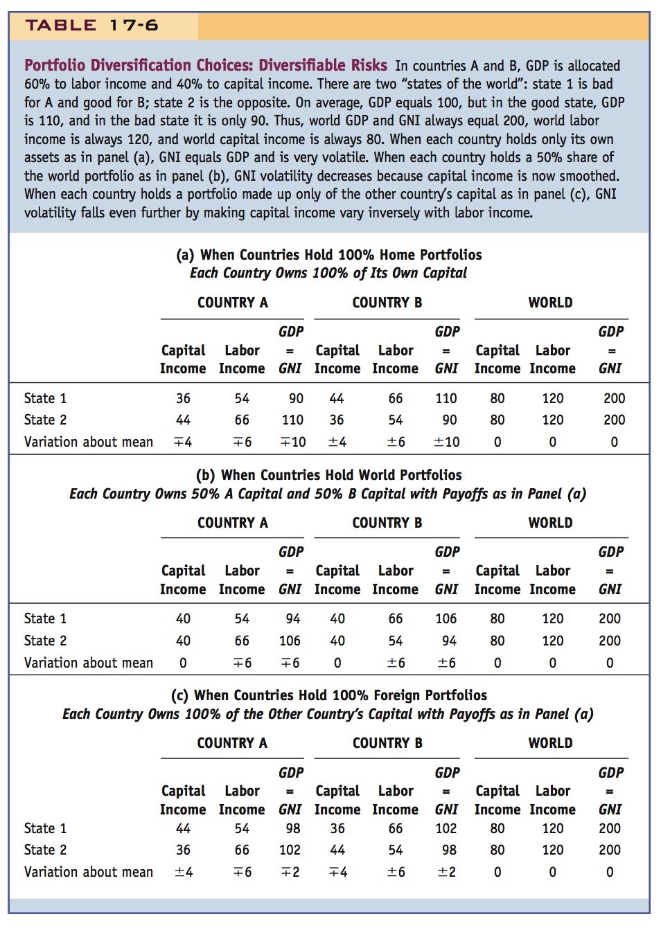
World Portfolios Notice that when one country’s capital income is up, the other’s is down. World GDP equals world GNI and is always 200. World labor income is always 120 and world capital income is always 80.
238
Emphasize the benefits of risk sharing.
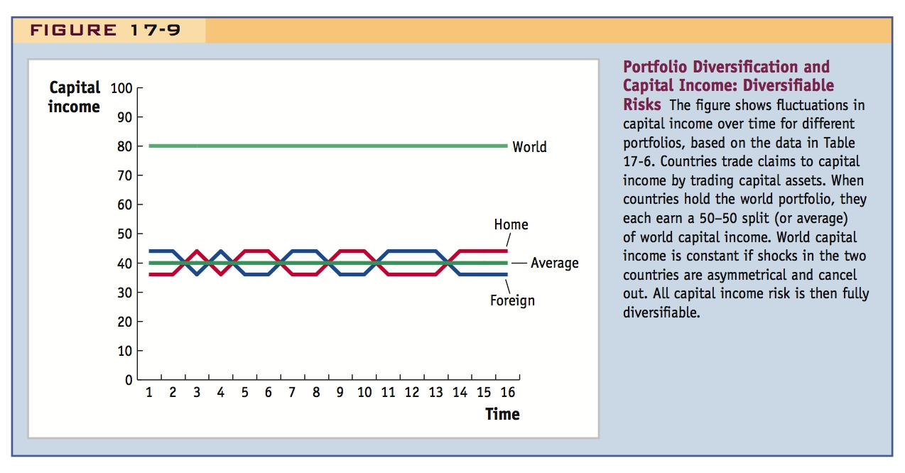
It is apparent from Figure 17-9 that the two countries can achieve partial income smoothing if they diversify their portfolios of capital assets. For example, each country could own half of the domestic capital stock, and half of the other country’s capital stock. Indeed, this is what standard portfolio theory says that investors should try to do. The results of this portfolio diversification are shown in Table 17-6, panel (b).
239
Now each country owns one-half of its own capital stock but sells the other half to the other country in exchange for half of the other country’s capital stock.23 Each country’s output or GDP is still as it was described in panel (a). But now country incomes or GNI can differ from their outputs or GDP. Owning 50% of the world portfolio means that each country has a capital income of 40 every period. However, labor income still varies between 54 and 66 in the bad and good states, so total income (and hence consumption) varies between 94 and 106. Thus, as Table 17-6, panel (b), shows, capital income for each country is smoothed at 40 units, the average of A and B capital income in panel (a), as also illustrated in Figure 17-9.
How does the balance of payments work when countries hold the world portfolio? Consider country A. In state 1 (bad for A, good for B), A’s income or GNI exceeds A’s output, GDP, by 4 (94 − 90 = +4). Where does the extra income come from? The extra is net factor income from abroad of +4. Why is it +4? This is precisely equal to the difference between the income earned on A’s external assets (50% of B’s payments to capital of 44 = 22) and the income paid on A’s external liabilities (50% of A’s payments to capital of 36 = 18). What does A do with that net factor income? A runs a trade balance of −4, which means that A can consume 94, even when its output is only 90. Adding the trade balance of −4 to net factor income from abroad of +4 means that the current account is 0, and there is still no need for any net borrowing or lending, as assumed. These flows are reversed in state 2 (which is good for A, bad for B).
Note that after diversification, income or GNI varies in A and B by plus or minus 6 (around a mean of 100), which is less than the range of plus or minus 10 seen in Table 17-6, panel (a). This is because 40% of income is capital income and so 40% of the A income fluctuation of 10 can be smoothed by the portfolio diversification.
240
Generalizing Let us try to generalize the concept of capital income smoothing through diversification. Consider the volatility of capital income by itself, in the example we have just studied. Each country’s payments to capital are volatile. A portfolio of 100% country A’s capital or 100% of country B’s capital has capital income that varies by plus or minus 4 (between 36 and 44). But a 50–50 mix of the two leaves the investor with a portfolio of minimum, zero volatility (it always pays 40).
Students should find the benefits intuitively appealing.
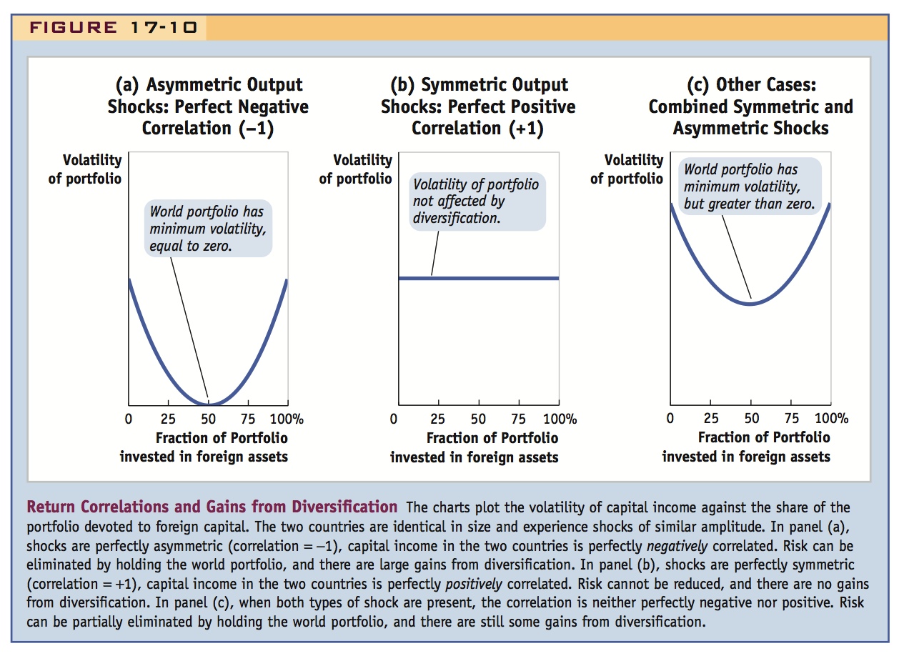
This outcome is summed up in Figure 17-10, panel (a), which refers to either country, A or B. There is an identical high level of capital income volatility when the country holds either a 100% home portfolio or a 100% foreign portfolio. However, holding a mix of the two reduces capital income volatility, and a minimum volatility of zero can be achieved by holding the 50–50 mix of the world capital income portfolio.
Again note that perfect risk sharing won't work if there are common, symmetric shocks.
To generalize this result to the real world, we need to recognize that not all shocks are asymmetric as we have assumed here. The outputs of countries A and B may not be equal and opposite (with correlation −1) as we have assumed here. In general, there will be some common shocks, which are identical shocks experienced by both countries. The impact of common shocks cannot be lessened or eliminated by any form of asset trade. For example, suppose we add an additional shock determined by two new states of the world, X and Y (these states of the world are independent of states of the world 1 and 2). We assume that in state X, the new shock adds five units to each country’s output; in state Y, it subtracts five units from each. There is no way to avoid this shock by portfolio diversification. The X-Y shocks in each country are perfectly positively correlated (correlation +1). If this were the only shock, the countries’ outputs would move up and down together and diversification would be pointless. This situation is shown in Figure 17-10, panel (b).
241
In the real world, any one country experiences some shocks that are correlated with those of other countries, either positively or negatively, and some that are uncorrelated. As long as some shocks are asymmetric, or country specific, and not common between the home and foreign country, then the two countries can take advantage of gains from the diversification of risk. In this more general case in which symmetric and asymmetric shocks are combined, as depicted in Figure 17-10, panel (c), holding a 100% portfolio of domestic (or foreign) assets generates a volatile income. But holding the 50–50 world portfolio will lower the volatility of income, albeit not all the way to zero (see the appendix at the end of the chapter for a detailed discussion).
Limits to Diversification: Capital Versus Labor Income As we saw in Table 17-6, panel (b), elimination of total income risk cannot be achieved by holding the world portfolio, even in the case of purely asymmetric shocks of capital assets. Why? Because labor income risk is not being shared. Admittedly, the same theory would apply if one could trade labor like an asset, but this is impossible because ownership rights to labor cannot be legally traded in the same way as one can trade capital or other property (that would be slavery).
Just as credit constraints may limit consumption smoothing, the presence of nontraded assets may limit risk sharing. Say that the absence of a market is making people worse off.
Although it is true that labor income risk (and hence GDP risk) may not be diversifiable through the trading of claims to labor assets or GDP, this is not quite the end of our story—in theory at least. We saw in Table 17-6, panel (a), that capital and labor income in each country are perfectly correlated in this example: a good state raises both capital and labor income, and a bad state lowers both. This is not implausible—in reality, shocks to production do tend to raise and lower incomes of capital and labor simultaneously. This means that, as a risk-sharing device, trading claims to capital income can substitute for trading claims to labor income.
To illustrate this, imagine an unrealistic scenario in which the residents of each country own no capital stock in their own country but own the entire capital stock of the other country. As shown in Table 17-6, panel (c), owning only the other country’s portfolio achieves more risk sharing than holding 50% of the world portfolio.
For example, when A is in the good state (state 2), A’s labor income is 66 but A’s capital income is 36 (assumed now to be 100% from B, which is in the bad state). This adds up to a portfolio of 102. In the bad state for A (state 2), A’s labor income is 54, but A’s capital income is 44 (from B, which is in a good state), for a total GNI of 98. So A’s income (and consumption) vary by plus or minus 2, between 98 and 102 in panel (c). Compare this fluctuation of ±2 around the mean of 100 to the fluctuations of ±10 (home portfolio) and ±6 (the world portfolio) in panels (a) and (b).
You can see how additional risk reduction has been achieved. A would like to own claims to 50% of B’s total income. It could achieve this by owning 50% of B’s capital and 50% of B’s labor. But labor can’t be owned, so A tries to get around the restriction of owning 0% of B’s labor by acquiring much more than 50% of B’s capital. Because labor’s share of income in both countries is more than half in this example—a realistic ratio—this strategy allows for the elimination of some, but not all, risk.
242
In reality, investors invest too little in foreign assets to fully capture the benefits of international diversification. They have a bias towards Home assets. Various explanations have been proposed (costs of acquiring foreign assets or information about them, asymmetries in consumption patterns, regulatory barriers, differences in corporate governance), but none is completely satisfactory. Perhaps the puzzle will disappear as financial globalization becomes more complete.
The Home Bias Puzzle
So much for theory. In practice, we do not observe countries owning foreign-biased portfolios or even the world portfolio. Countries tend to own portfolios that suffer from a strong home bias, a tendency of investors to devote a disproportionate fraction of their wealth to assets from their own home country, when a more globally diversified portfolio might protect them better from risk.
To illustrate this, economist Karen Lewis compared the risk and return for sample portfolios from which U.S. investors could have chosen for the period 1970 to 1996. She imagined an experiment in which some assets are allocated to a domestic portfolio (the S&P 500) and the remainder to an overseas portfolio (Morgan Stanley’s EAFE fund). In this stylized problem, the question is what weight to put on each portfolio, when the weights must sum to 100%. In reality, U.S. investors picked a weight of about 8% on foreign assets. Was this a smart choice?
Figure 17-11 shows the risk and return for every possible weight between 0% and 100%. Return is measured by the mean rate of return (annualized percent per year); risk is measured by the standard deviation of the return (its root mean square deviation from its mean).
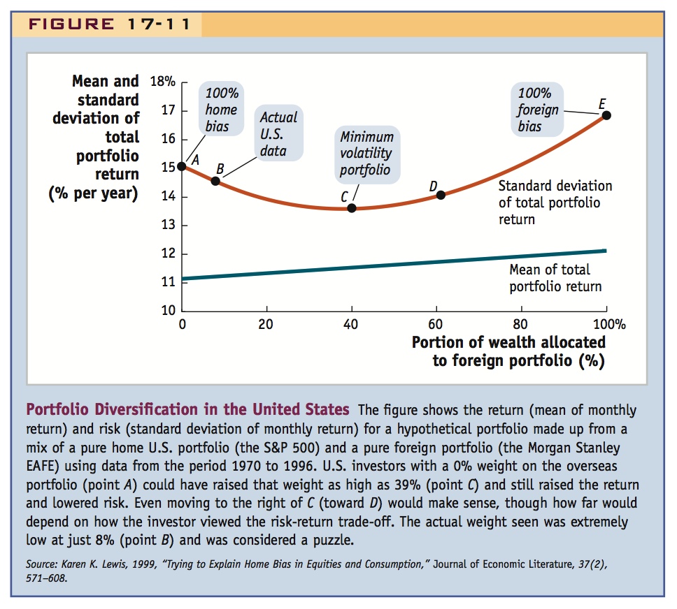
With regard to returns, the foreign portfolio had a slightly higher average return than the home portfolio during this period, so increasing the weight in the foreign portfolio would have increased the returns: the mean return line slopes up slightly from left to right. What about risk? A 100% foreign portfolio (point E) would have generated higher risk than the home U.S. portfolio (point A); thus, E is above A. However, we know that some mix of the two portfolios ought to produce a lower volatility than either extreme because the two returns are not perfectly correlated. This minimum volatility will not be zero because there are some undiversifiable, symmetric shocks, but it will be lower than the volatility of the 100% home and 100% foreign portfolios: overseas and domestic returns are not perfectly correlated, implying that substantial country-specific diversifiable risks exist.
243
In fact, Lewis showed that a U.S. investor with a 0% weight on the overseas portfolio (point A) could have raised that weight to as much as 39% (point C), while simultaneously raising the average of her total return and lowering its risk. Even moving to the right of C (toward D) would make sense, though how far would depend on how the investor viewed the risk-return trade-off. Choosing a weight as low as 8% (point B) would seem to be a puzzle.
Broadly speaking, economists have had one of two reactions to the emergence of the “home bias puzzle” in the 1990s. One is to propose many different theories to explain it away: Perhaps it is costly to acquire foreign assets, or get information about them? Perhaps there are asymmetries between home and foreign countries’ consumption patterns (due to nontraded goods or trade frictions or even tastes) that make domestic assets a better hedge against domestic consumption risk? Perhaps home investors worry about regulatory barriers and the problems of corporate governance in foreign markets? These and many other solutions have been tried in extremely complex economic models, but none has been judged a complete success.
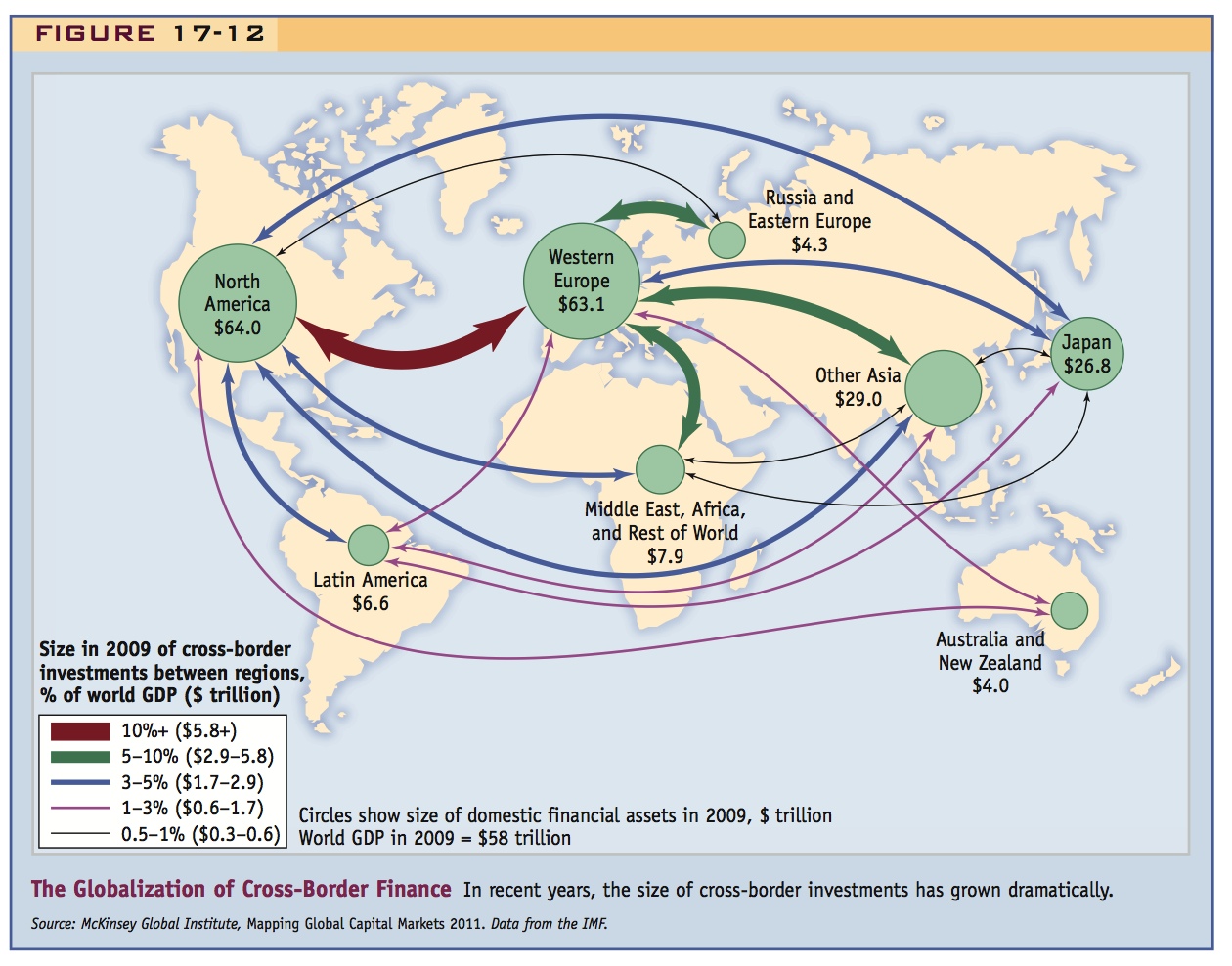
The other reaction of economists has been to look at the evidence of home bias in the period from the 1970s to the 1990s (the period of the Lewis study) as a legacy of the pronounced deglobalization of financial markets in the postwar period that might slowly disappear. Recent evidence suggests that this might be happening to some degree. There has been a dramatic increase in overseas equity investments in the last 40 years, with a very strong upward trend after 1985 in IMF data. For example, in the United States, the foreign share of the U.S. equity portfolio had risen to 12% by 2001 and 28% in 2010. Over the same period, the U.K. portfolio saw its foreign equity share rise from 28% to 50%. Figure 17-12 shows the massive extent of cross-border holdings of assets in today’s global economy. Furthermore, these figures might understate the true extent to which residents have diversified away from home capital because many large multinational firms have capital income streams that flow from operations in many countries. For example, an American purchasing a share of Intel or Ford, or a Briton purchasing a share of BP, or a Japanese person purchasing a share of Sony, is really purchasing shares of income streams from the globally diversified operations of these companies. Technically, Intel is recorded in the data as a 100% U.S. “home” stock, but this makes the home bias puzzle look much worse than it really is because investors do seem to invest heavily in firms such as these that provide an indirect foreign exposure.24
244
Recent trends in diversification within portfolios and within companies may mean that even if the puzzle cannot be explained away, perhaps it will gradually go away.
Ask the students what might prevent them from wanting to diversify their portfolios to include more foreign assets.
Summary: Don’t Put All Your Eggs in One Basket
2. Summary: Don’t Put All of Your Eggs in One Basket
International diversification should yield substantial benefits by reducing consumption risk. However, investors seem to have a bias towards domestic assets, and don’t fully exploit these potential benefits.
Another useful phrase that will stick in students' minds.
If countries were able to borrow and lend without limit or restrictions in an efficient global capital market, our discussions of consumption smoothing and efficient investment would seem to suggest that they should be able to cope quite well with the array of possible shocks, in order to smooth consumption. In reality, as the evidence shows, countries are not able to fully exploit the intertemporal borrowing mechanism.
In this environment, diversification of income risk through the international trading of assets can deliver substantial benefits. In theory, if countries were able to pool their income streams and take shares from that common pool of income, all country-specific shocks would be averaged out, leaving countries exposed only to common global shocks to income, the sole remaining undiversifiable shocks that cannot be avoided.
Financial openness allows countries—like households—to follow the old adage “Don’t put all your eggs in one basket.” The lesson here has a simple household analogy. Think of a self-employed person who owns a ski shop. If the only capital she owns is her own business capital, then her capital income and labor income move together, and go up in good times (winter) and down in bad times (summer). Her total income could be smoothed if she sold some stock in her company and used the proceeds to buy stock in another company that faced asymmetric shocks (a surf shop, perhaps).
245
In practice, however, risk sharing through asset trade is limited. For one thing, the number of assets is limited. The market for claims to capital income is incomplete because not all capital assets are traded (e.g., many firms are privately held and are not listed on stock markets), and trade in labor assets is legally prohibited. Moreover, even with the traded assets available, investors have shown very little inclination to invest their wealth outside their own country, although that may be slowly changing in an environment of ongoing financial globalization.