3 Goods and Forex Market Equilibria: Deriving the IS Curve

We have made an important first step in our study of the short-run behavior of exchange rates and output. Our analysis of demand shows how the level of output adjusts to ensure a goods market equilibrium, given the levels of each component of demand. Each component, in turn, has its own particular determinants, and we have examined how shifts in these determinants (or in other exogenous factors) might shift the level of demand and, hence, change the equilibrium level of output.

But there is more than one market in the economy, and a general equilibrium requires equilibrium in all markets—that is, equilibrium in the goods market, the money market, and the forex market. We need to bring all three markets into the analysis, and we do that next by developing a tool of macroeconomic analysis known as the IS-LM diagram. A version of this may be familiar to you from the study of closed-economy macroeconomics, but in this chapter we develop a variant of this approach for an open economy.

Analyzing equilibria in three markets simultaneously is a difficult task, but it is made more manageable by proceeding one step at a time using familiar tools. Our first step builds on the Keynesian cross depiction of goods market equilibrium developed in the last section and then adds on the depiction of forex market equilibrium that we developed in the earlier exchange rate chapters.

Equilibrium in Two Markets

We begin by defining the IS curve, which is one part of the IS-LM diagram.

The IS curve shows combinations of output Y and the interest rate i for which the goods and forex markets are in equilibrium.

In Figure 18-8, panel (b), we derive the IS curve by using the Keynesian cross in panel (a) to analyze goods market equilibrium. In panel (c), we impose the uncovered interest parity relationship that ensures the forex market is in equilibrium.

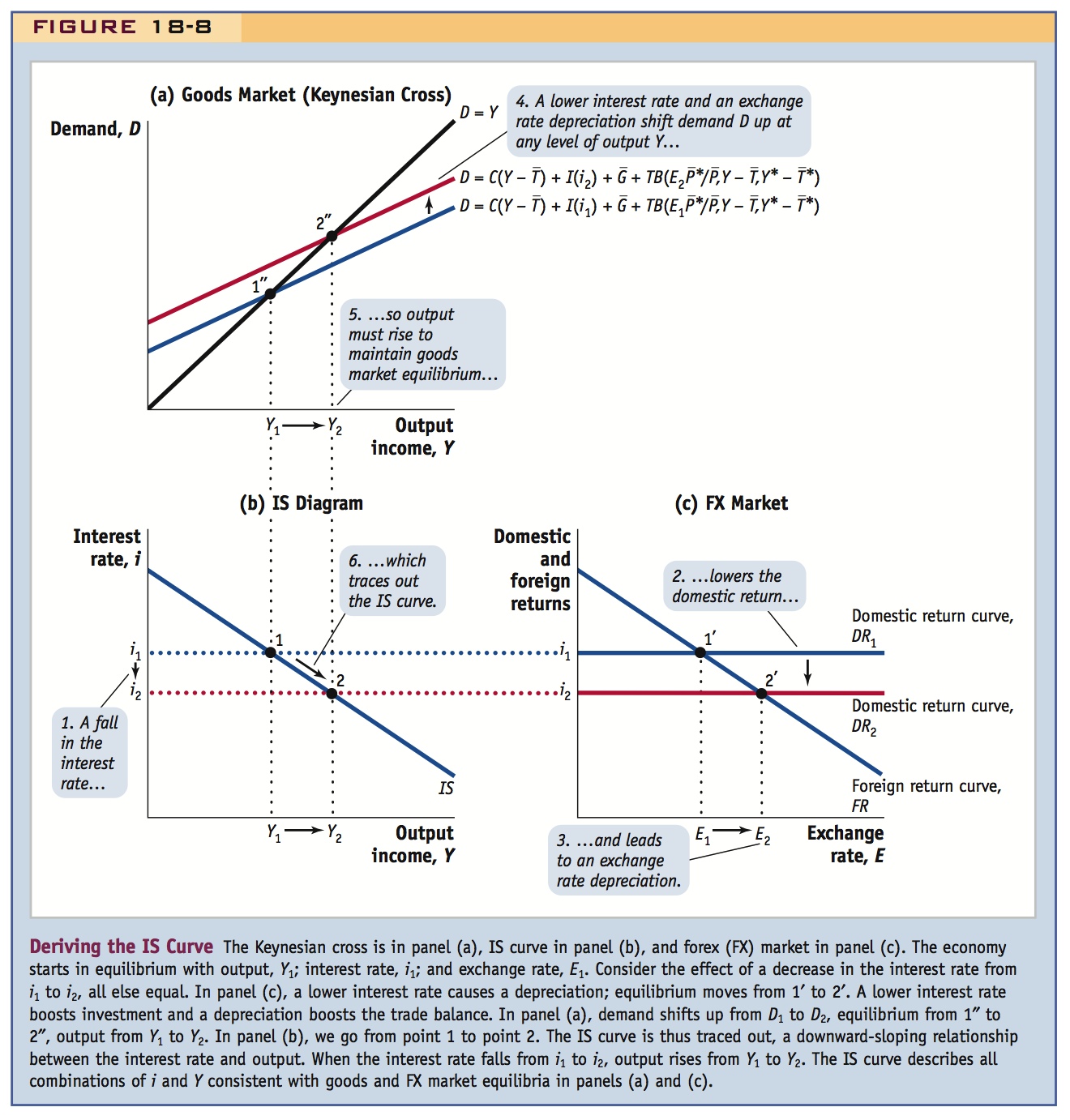
Before we continue, let’s take a closer look at why the various graphs in this figure are oriented as they are. The Keynesian cross in panel (a) and the IS diagram in panel (b) share a common horizontal axis, the level of output or income. Hence, these figures are arranged one above the other so that these common output axes line up.

The forex market in panel (c) and the IS diagram in panel (b) share a common vertical axis, the level of the domestic interest rate. Hence, these figures are arranged side by side so that these common interest rate axes line up.

We thus know that if output Y is at a level consistent with demand equals supply, shown in the Keynesian cross in panel (a), and if the interest rate i is at a level consistent with uncovered interest parity, shown in the forex market in panel (c), then in panel (b), then we must have a combination of Y and i that is consistent with equilibrium in both goods and forex markets.

Forex Market Recap

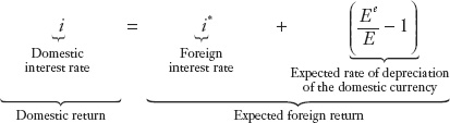
In earlier chapters we learned that the forex market is in equilibrium when the expected returns expressed in domestic currency are the same on foreign and domestic interest-bearing (money market) bank deposits. Equation (4-1) described this condition, known as uncovered interest parity (UIP), where home and foreign currencies corresponded to the dollar and the euro; for any currency pair we can write, similarly:

The expected return on the foreign deposit measured in home currency equals the foreign interest rate plus the expected rate of depreciation of the home currency.

Taking the foreign interest rate i^* and expectations of the future exchange rate E^e as given, we know that the right-hand side of this expression decreases as E increases: the intuition for this is that the more expensive it is to purchase foreign currency today, the lower the expected return must be, all else equal.

The inverse relationship between E and the expected foreign return on the right-hand side of the previous equation is shown by the downward-sloping FR (foreign returns) line in panel (c) of Figure 18-8. The domestic return DR is the horizontal line corresponding to the level of the domestic interest rate i.

Deriving the IS Curve

Using the setup in Figure 18-8, we can now derive the shape of the IS curve by considering how changes in the interest rate affect output if the goods and forex markets are to remain in equilibrium.

Initial Equilibrium Let us suppose that the goods market and forex markets are initially in equilibrium at an interest rate i₁, an output or income level Y₁, and an exchange rate E₁.

In panel (a) by assumption, at an output level Y₁, demand equals supply, so the output level Y₁ must correspond to the point 1″, which is at the intersection of the Keynesian cross, and the figure is drawn accordingly.

In panel (c) by assumption, at an interest rate i₁ and an exchange rate E₁, the domestic and foreign returns must be equal, so this must be the point 1′, which is at the intersection of the DR₁ and FR curves, and the figure is drawn accordingly.

Finally, in panel (b) by assumption, at an interest rate i₁ and an output level Y₁, both goods and forex markets are in equilibrium. Thus, the point 1 is on the IS curve, by definition.

Lines are drawn joining the equal output levels Y₁ in panels (a) and (b). The domestic return line DR₁ traces out the home interest rate level from panel (b) across to panel (c).

A Fall in the Interest Rate Now in Figure 18-8, let us suppose that the home interest rate falls from i₁ to i₂. What happens to equilibria in the good and forex markets?

We first look at the forex market in panel (c). From our analysis of UIP in earlier chapters we know that when the home interest rate falls, domestic deposits have a lower return and look less attractive to investors. To maintain forex market equilibrium, the exchange rate must rise (the home currency must depreciate) until domestic and foreign returns are once again equal. In our example, when the home interest rate falls to i₂, the exchange rate must rise from E₁ to E₂ to equalize FR and DR₂ and restore equilibrium in the forex market at point 2′.

How do the changes in the home interest rate and the exchange rate affect demand? As shown in panel (a), demand will increase (shift up) for two reasons, as we learned earlier in this chapter.

First, when the domestic interest rate falls, firms are willing to engage in more investment projects, and their increased investment augments demand. The increase in investment, all else equal, directly increases demand D at any level of output Y.

Second, the exchange rate E has risen (depreciated). Because prices are sticky in the short run, this rise in the nominal exchange rate E also causes a rise in the real exchange rate . That is, the nominal depreciation causes a real depreciation. This increases demand D via expenditure switching. At any level of output Y consumers switch expenditure from relatively more expensive foreign goods toward relatively less expensive domestic goods. Thus, the fall in the interest rate indirectly boosts demand via exchange rate effects felt through the trade balance TB.

One important observation is in order: in an open economy, the phenomenon of expenditure switching operates as an additional element in demand that is not present in a closed economy. In an open economy, lower interest rates stimulate demand through the traditional closed-economy investment channel and through the trade balance. The trade balance effect occurs because lower interest rates cause a nominal depreciation, which in the short run is also a real depreciation, which stimulates external demand via the trade balance.

To summarize, panel (a) shows clearly that in response to a decrease in the interest rate, demand has shifted up to D₂ and the Keynesian cross goods market equilibrium is restored by a rise in output to Y₂, which corresponds to point 2″.

In panel (b), we can now derive the shape of the IS curve. At an interest rate i₁ and output level Y₁ and at an interest rate i₂ and an output level Y₂, both the goods and forex markets are in equilibrium. We have now derived the shape of the IS curve, which describes goods and forex market equilibrium. When the interest rate falls from i₁ to i₂, output rises from Y₁ to Y₂. The IS curve is downward sloping, which illustrates the negative relationship between the interest rate i and output Y.

Factors That Shift the IS Curve

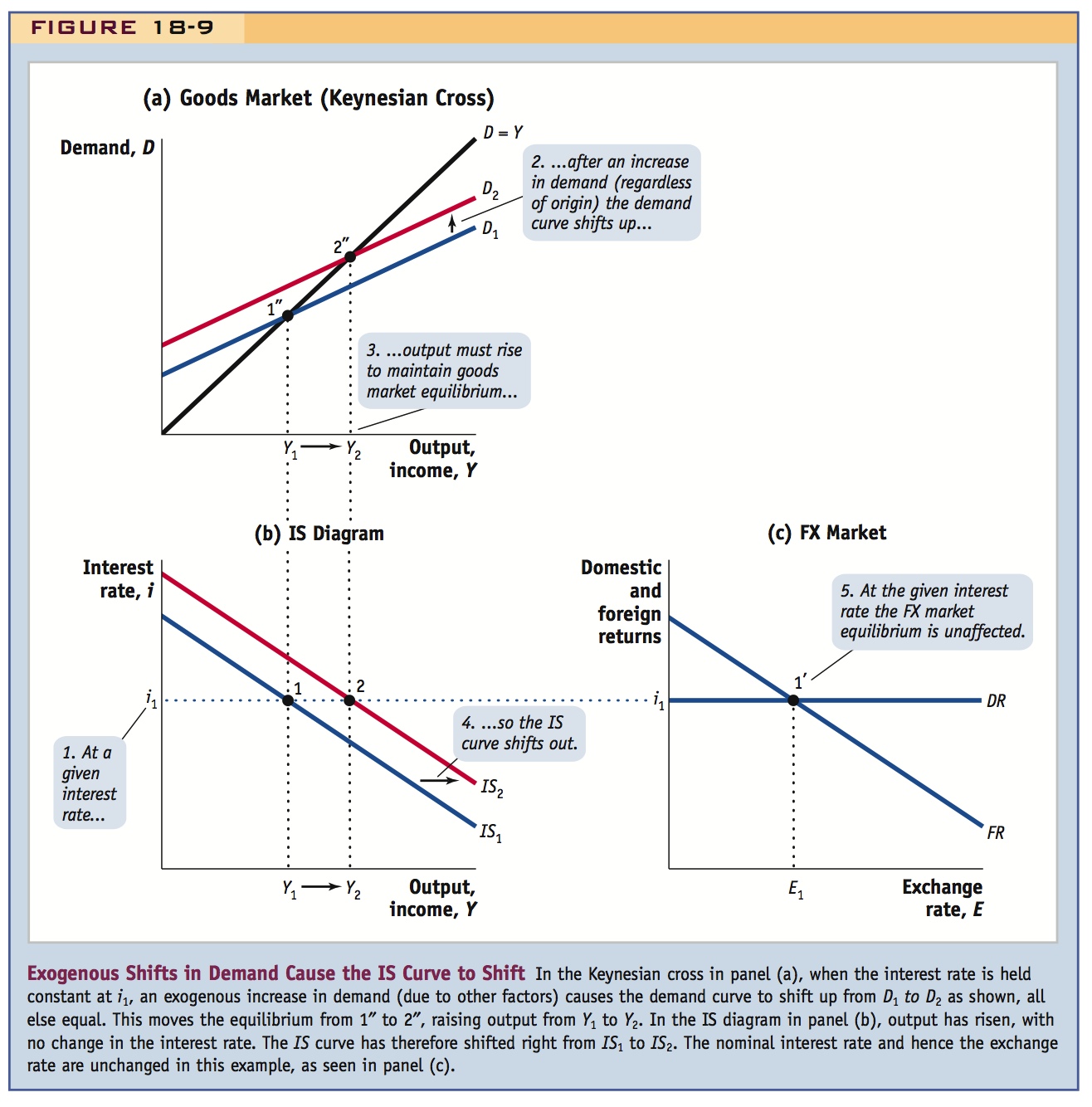
In deriving the IS curve, we treated various demand factors as exogenous, including fiscal policy, price levels, and the exchange rate. If any factors other than the interest rate and output change, the position of the IS curve would have to change. These effects are central in any analysis of changes in an economy’s equilibrium. We now explore several changes that result in an increase in demand, that is, an upward shift in the demand curve in Figure 18-9, panel (a). (A decrease in demand would result from changes in the opposite direction.)

• A change in government spending. If demand shifts up because of a rise in , a fiscal expansion, all else equal, what happens to the IS curve? The initial equilibrium point (Y₁, i₁) would no longer be a goods market equilibrium: if the interest rate is unchanged at i₁, then I is unchanged, as are the exchange rate E and hence TB. Yet demand has risen due to the change in G. That demand has to be satisfied somehow, so more output has to be produced. Some—but not all—of that extra output will be consumed, but the rest can meet the extra demand generated by the rise in government spending. At the interest rate i₁, output must rise to Y₂ for the goods market to once again be in equilibrium. Thus, the IS curve must shift right as shown in Figure 18-9, panel (b).

The lesson: a rise in government spending shifts the IS curve out.

• A change in taxes. Suppose taxes were to decrease. With all other factors remaining unchanged, this tax cut makes demand shift up by boosting private consumption, all else equal. We assume that the interest rate i₁, the exchange rate E₁, and government’s spending policy are all fixed. Thus, neither I nor TB nor G change. With an excess of demand, supply has to rise, so output must again increase to Y₂ and the IS curve shifts right.

The lesson: a reduction in taxes shifts the IS curve out.

• A change in the foreign interest rate or expected future exchange rate. A rise in the foreign interest rate i^* or a rise in the future expected exchange rate E^e causes a depreciation of the home currency, all else equal (recall that in the forex market, the FR curve shifts out because the return on foreign deposits has increased; if the home interest rate is unchanged, E must rise). A rise in E causes the real exchange rate to depreciate, because prices are sticky. As a result, TB rises via expenditure switching, and demand increases. Because C, I, and G do not change, there is an excess of demand, and supply has to rise to restore equilibrium. Output Y increases, and the IS curve shifts right.

The lesson: an increase in the foreign return (via i^* or E^e) shifts the IS curve out.

• A change in the home or foreign price level. If prices are flexible, then a rise in foreign prices or a fall in domestic prices causes a home real depreciation, raising . This real depreciation causes TB to rise and, all else equal, demand will rise to a position like D₂. With an excess of demand, supply has to rise to restore equilibrium. Output Y must increase, and the IS curve shifts right.

The lesson: an increase P^* or a decrease in P shifts the IS curve out.

These examples show that the position of the IS curve depends on various factors that we treat as given (or exogenous). We may write this observation using the notation

There are many other exogenous shocks to the economy that can be analyzed in a similar fashion—for example, a sudden exogenous change in consumption, investment, or the trade balance. How will the IS curve react in each case? You may have detected a pattern from the preceding discussion.

The general rule is as follows: any type of shock that increases demand at a given level of output will shift the IS curve to the right; any shock that decreases demand will shift the IS curve down.

Summing Up the IS Curve

When prices are sticky, the IS curve summarizes the relationship between output Y and the interest rate i necessary to keep the goods and forex markets in short-run equilibrium. The IS curve is downward-sloping. Why? Lower interest rates stimulate demand via the investment channel and, through exchange rate depreciation, via the trade balance. Higher demand can be satisfied in the short run only by higher output. Thus, when the interest rate falls, output rises, and the economy moves along the IS curve.

As for shifts in the IS curve, we have found that any factor which increases demand D at a given home interest rate i must cause the demand curve to shift up, leading to higher output Y and, as a result, an outward shift in the IS curve.

To conclude, the main factors that shift the IS curve out can be summed up as follows:

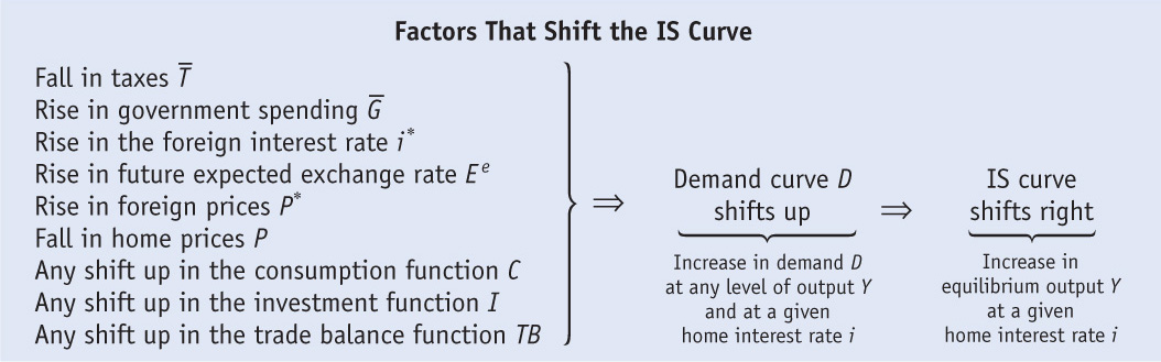
The opposite changes lead to a decrease in demand and shift the demand curve down and the IS curve to the left.