5 The Short-Run IS-LM-FX Model of an Open Economy

We are now in a position to fully characterize an open economy that is in equilibrium in goods, money, and forex markets, as shown in Figure 18-12. This IS-LM-FX figure combines the goods market (the IS curve), the money market (the LM curve), and the forex (FX) market diagrams.

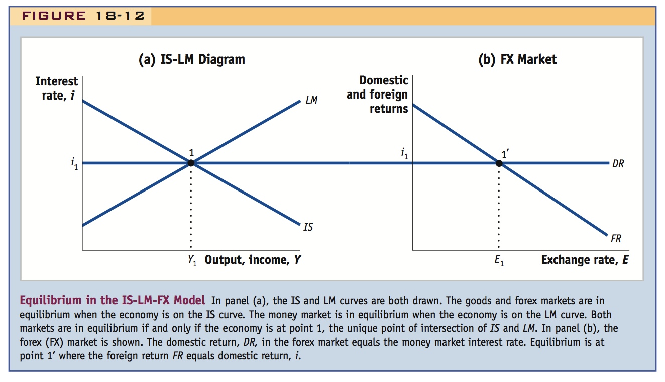
The IS and LM curves are both drawn in panel (a). The goods and forex markets are in equilibrium if and only if the economy is on the IS curve. The money market is in equilibrium if and only if the economy is on the LM curve. Thus, all three markets are in equilibrium if and only if the economy is at point 1, where IS and LM intersect.

The forex market, or FX market, is drawn in panel (b). The domestic return DR in the forex market equals the money market interest rate. Equilibrium is at point 1′ where the foreign return FR is equal to domestic return i.

In the remainder of this chapter, and in the rest of this book, we make extensive use of this two-panel IS-LM-FX diagram of the open-economy equilibrium to analyze the short-run response of an open economy to various types of shocks. In particular, we look at how government policies affect the economy and the extent to which they can be employed to enhance macroeconomic performance and stability.

Macroeconomic Policies in the Short Run

Now that we understand the open-economy IS-LM-FX model and all the factors that influence an economy’s short-run equilibrium, we can use the model to look at how a nation’s key macroeconomic variables (output, exchange rates, trade balance) are affected in the short run by changes in government macroeconomic policies.

We focus on the two main policy actions: changes in monetary policy, implemented through changes in the money supply, and changes in fiscal policy, involving changes in government spending or taxes. Of particular interest is the question of whether governments can use such policies to insulate the economy from fluctuations in output.

We will see that the impact of these policies is profoundly affected by a nation’s choice of exchange rate regime, and we will consider the two polar cases of fixed and floating exchange rates. Many countries are on some kind of flexible exchange rate regime and many are on some kind of fixed regime, so considering policy effects under both fixed and floating systems is essential.

The key assumptions of this section are as follows. The economy begins in a state of long-run equilibrium. We then consider policy changes in the home economy, assuming that conditions in the foreign economy (i.e., the rest of the world) are unchanged. The home economy is subject to the usual short-run assumption of a sticky price level at home and abroad. Furthermore, we assume that the forex market operates freely and unrestricted by capital controls and that the exchange rate is determined by market forces.

Temporary Policies, Unchanged Expectations Finally, we examine only temporary changes in policies. We will assume that long-run expectations about the future state of the economy are unaffected by the policy changes. In particular, the future expected exchange rate E^e is held fixed. The reason for studying temporary policies is that we are primarily interested in how governments use fiscal and monetary policies to handle temporary shocks and business cycles in the short run, and our model is applicable only in the short run.2

The key lesson of this section is that policies matter and can have significant macroeconomic effects in the short run. Moreover, their impacts depend in a big way on the type of exchange rate regime in place. Once we understand these linkages, we will better understand the contentious and ongoing debates about exchange rates and macroeconomic policies, including the never-ending arguments over the merits of fixed and floating exchange rates (a topic covered in detail in the next chapter).

Monetary Policy Under Floating Exchange Rates

In this policy experiment, we consider a temporary monetary expansion in the home country when the exchange rate is allowed to float. Because the expansion is not permanent, we assume there is no change in long-run expectations so that the expected future exchange rate remains steady at E^e. This means that there is no change in the expected foreign return curve in the forex market.

Figure 18-13 illustrates the predictions of the model. In panel (a) in the IS-LM diagram, the goods and money markets are initially in equilibrium at point 1. The interest rate in the money market is also the domestic return DR₁ that prevails in the forex market. In panel (b), the forex market is initially in equilibrium at point 1′.

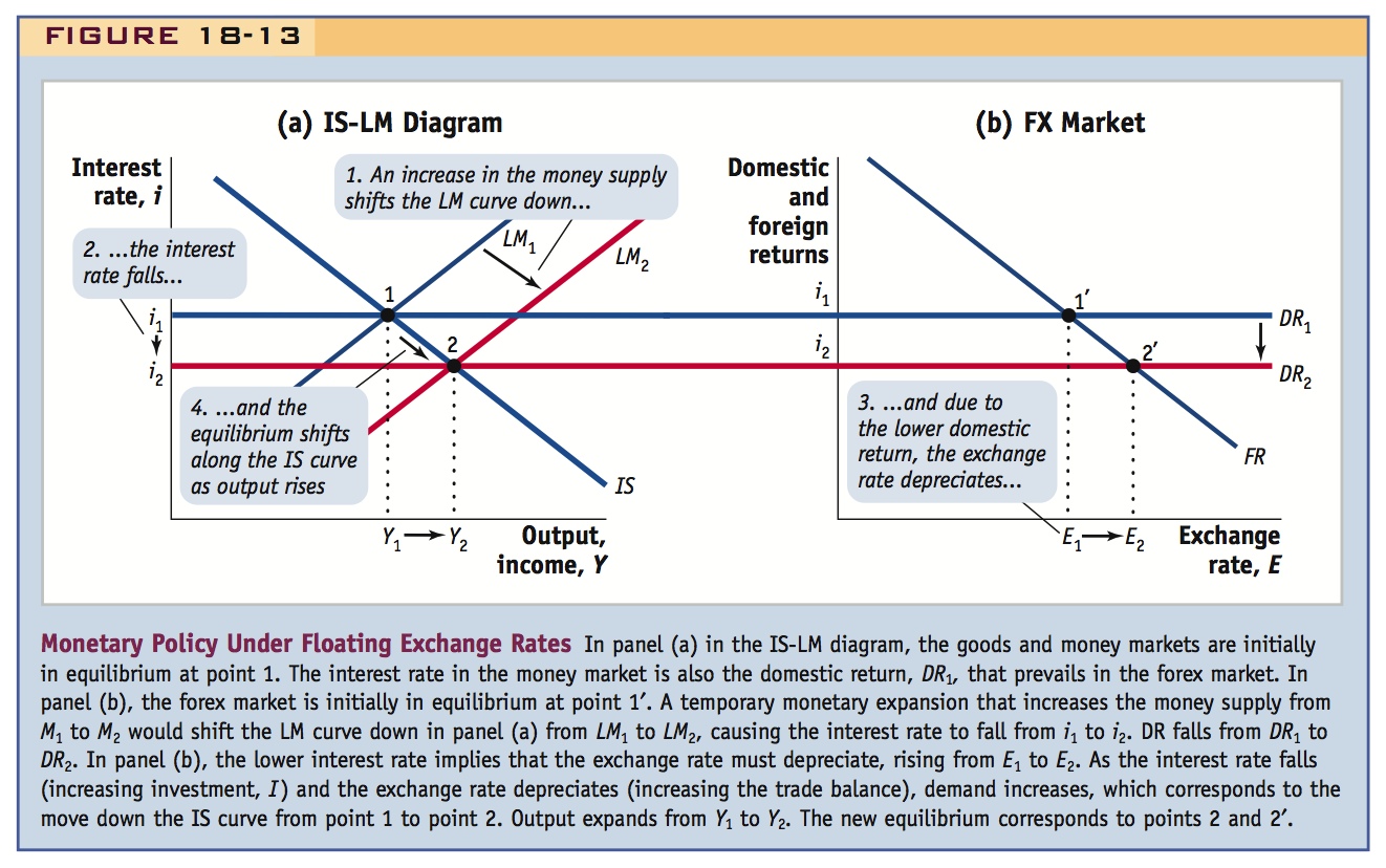
A temporary monetary expansion that increases the money supply from M₁ to M₂ would shift the LM curve to the right in panel (a) from LM₁ to LM₂, causing the interest rate to fall from i₁ to i₂. The domestic return falls from DR₁ to DR₂. In panel (b), the lower interest rate would imply that the exchange rate must depreciate, rising from E₁ to E₂. As the interest rate falls (increasing investment I) and the exchange rate depreciates (increasing the trade balance), demand increases, which corresponds to the move down the IS curve from point 1 to point 2. Output expands from Y₁ to Y₂. The new equilibrium corresponds to points 2 and 2′.

The intuition for this result is as follows: monetary expansion tends to lower the home interest rate, all else equal. A lower interest rate stimulates demand in two ways. First, directly in the goods market, it causes investment demand I to increase. Second, indirectly, it causes the exchange rate to depreciate in the forex market, which in turn causes expenditure switching in the goods market, which causes the trade balance TB to increase. Both I and TB are sources of demand and both increase.

To sum up: a temporary monetary expansion under floating exchange rates is effective in combating economic downturns because it boosts output. It also lowers the home interest rate, and causes a depreciation of the exchange rate. What happens to the trade balance cannot be predicted with certainty: increased home output will decrease the trade balance as the demand for imports will rise, but the real depreciation will increase the trade balance, because expenditure switching will tend to raise exports and diminish imports. In practice, economists tend to assume that the latter outweighs the former, so a temporary expansion of the money supply is usually predicted to increase the trade balance. (The case of a temporary contraction of monetary policy has opposite effects. As an exercise, work through this case using the same graphical apparatus.)

Monetary Policy Under Fixed Exchange Rates

Now let’s look at what happens when a temporary monetary expansion occurs when the home country fixes its exchange rate with the foreign country at . The key to understanding this experiment is to recall the uncovered interest parity condition: the home interest rate must equal the foreign interest rate under a fixed exchange rate.

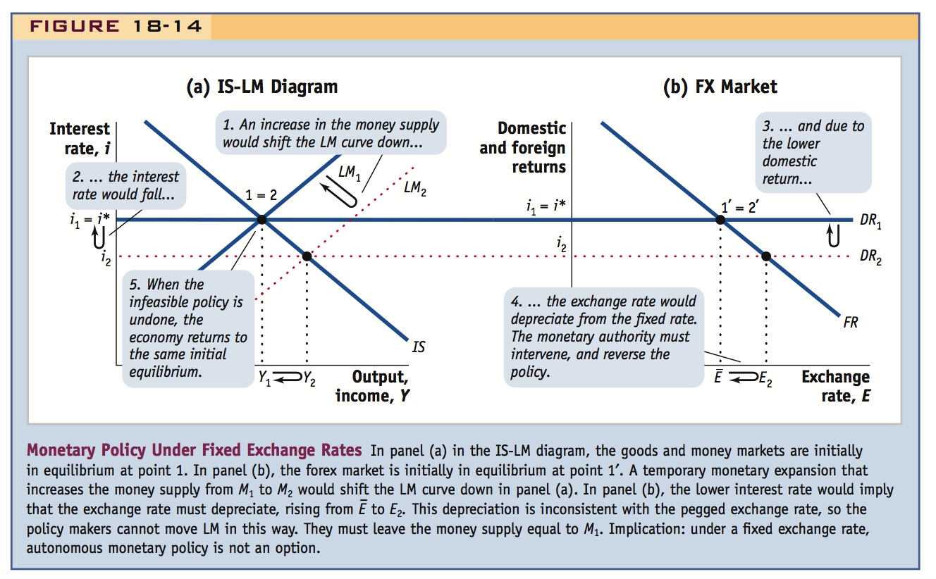
Figure 18-14 puts the model to work. In panel (a) in the IS-LM diagram, the goods and money markets are initially in equilibrium at point 1. In panel (b), the forex market is initially in equilibrium at point 1′.

A temporary monetary expansion that increases the money supply from M₁ to M₂ would shift the LM curve down and to the right in panel (a), and the interest rate would tend to fall, as we have just seen. In panel (b), the lower interest rate would imply that the exchange rate would tend to rise or depreciate toward E₂. This is inconsistent with the pegged exchange rate , so the policy makers cannot alter monetary policy and shift the LM curve in this way. They must leave the money supply equal to M₁ and the economy cannot deviate from its initial equilibrium.

This example illustrates a key lesson: under a fixed exchange rate, autonomous monetary policy is not an option. What is going on? Remember that under a fixed exchange rate, the home interest rate must exactly equal the foreign interest rate, i = i^*, according to the uncovered interest parity condition. Any shift in the LM curve would violate this restriction and break the fixed exchange rate.

To sum up: monetary policy under fixed exchange rates is impossible to undertake. Fixing the exchange rate means giving up monetary policy autonomy. In an earlier chapter, we learned about the trilemma: countries cannot simultaneously allow capital mobility, maintain fixed exchange rates, and pursue an autonomous monetary policy. We have now just seen the trilemma at work in the IS-LM-FX framework. By illustrating a potential benefit of autonomous monetary policy (the ability to use monetary policy to increase output), the model clearly exposes one of the major costs of fixed exchange rates. Monetary policy, which in principle could be used to influence the economy in the short run, is ruled out by a fixed exchange rate.

Fiscal Policy Under Floating Exchange Rates

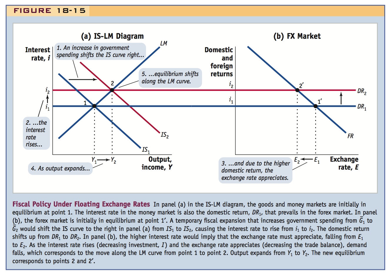
We now turn to fiscal policy under a floating exchange rate. In this example, we consider a temporary increase in government spending from to in the home economy. Again, the effect is not permanent, so there are no changes in long-run expectations, and in particular the expected future exchange rate remains steady at E^e. Figure 18-15 shows what happens in our model. In panel (a) in the IS-LM diagram, the goods and money markets are initially in equilibrium at point 1. The interest rate in the money market is also the domestic return DR₁ that prevails in the forex market. In panel (b), the forex market is initially in equilibrium at point 1′.

A temporary fiscal expansion that increases government spending from to would shift the IS curve to the right in panel (a) from IS₁ to IS₂, causing the interest rate to rise from i₁ to i₂. The domestic return rises from DR₁ to DR₂. In panel (b), the higher interest rate would imply that the exchange rate must appreciate, falling from E₁ to E₂. As the interest rate rises (decreasing investment I) and the exchange rate appreciates (decreasing the trade balance TB), demand still tends to rise overall as government spending increases, which corresponds to the move up the LM curve from point 1 to point 2. Output expands from Y₁ to Y₂. The new equilibrium is at points 2 and 2′.

What is happening here? The fiscal expansion raises output as the IS curve shifts right. But the increases in output will raise interest rates, all else equal, given a fixed money supply. The resulting higher interest rates will reduce the investment component of demand, and this limits the rise in demand to less than the increase in government spending. This impact of fiscal expansion on investment is often referred to as crowding out by economists.

The higher interest rate also causes the home currency to appreciate. As home consumers switch their consumption to now less expensive foreign goods, the trade balance will fall. Thus, the higher interest rate also (indirectly) leads to a crowding out of net exports, and this too limits the rise in output to less than the increase in government spending. Thus, in an open economy, fiscal expansion not only crowds out investment (by raising the interest rate) but also crowds out net exports (by causing the exchange rate to appreciate).

To sum up: a temporary expansion of fiscal policy under floating exchange rates is effective. It raises output at home, raises the interest rate, causes an appreciation of the exchange rate, and decreases the trade balance. (A temporary contraction of fiscal policy has opposite effects. As an exercise, work through the contraction case using the same graphical apparatus.)

Fiscal Policy Under Fixed Exchange Rates

Now let’s see how the outcomes differ when the home country pegs its exchange rate with respect to the foreign country at . The key is to recall the parity condition: the home interest rate must remain exactly equal to the foreign interest rate for the peg to hold.

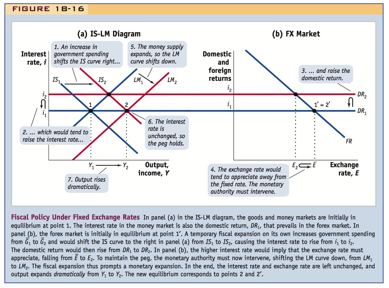
Figure 18-16 shows what happens in this case. In panel (a) in the IS-LM diagram, the goods and money markets are initially in equilibrium at point 1. The interest rate in the money market is also the domestic return DR₁ that prevails in the forex market. In panel (b), the forex market is initially in equilibrium at point 1′.

A temporary fiscal expansion that increases government spending from to would shift the IS curve to the right in panel (a) from IS₁ to IS₂, causing the interest rate to rise from i₁ to i₂. The domestic return would rise from DR₁ to DR₂. In panel (b), the higher interest rate would imply that the exchange rate must appreciate, falling from to E₂. To maintain the peg, the monetary authority must intervene, shifting the LM curve to the right also, from LM₁ to LM₂. The fiscal expansion thus prompts a monetary expansion. In the end, the interest rate and exchange rate are left unchanged, and output expands dramatically from Y₁ to Y₂. The new equilibrium corresponds to points 2 and 2′.

What is happening here? From the last example, we know that there is appreciation pressure associated with a fiscal expansion if the currency is allowed to float. To maintain the peg, the monetary authority must immediately alter its monetary policy at the very moment the fiscal expansion occurs so that the LM curve shifts from LM₁ to LM₂. The way to do this is to expand the money supply, and this generates pressure for depreciation, offsetting the appreciation pressure. If the monetary authority pulls this off, the market exchange rate will stay at the initial pegged level .

Thus, when a country is operating under a fixed exchange, fiscal policy is super-effective because any fiscal expansion by the government forces an immediate monetary expansion by the central bank to keep the exchange rate steady. The double, and simultaneous, expansion of demand by the fiscal and monetary authorities imposes a huge stimulus on the economy, and output rises from Y₁ to Y₂ (beyond the level achieved by the same fiscal expansion under a floating exchange rate).

To sum up: a temporary expansion of fiscal policy under fixed exchange rates raises output at home by a considerable amount. (The case of a temporary contraction of fiscal policy would have similar but opposite effects. As an exercise, work through this case using the same graphical apparatus.)

Summary

We have now examined the operation of fiscal and monetary policies under both fixed and flexible exchange rates and have seen how the effects of these policies differ dramatically depending on the exchange rate regime. The outcomes can be summarized as follows:

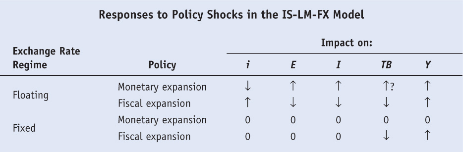
In this table, an up arrow ↑ indicates that the variable rises; a down arrow ↓ indicates that the variables falls; and a zero indicates no effect. The effects would be reversed for contractionary policies. The row of zeros for monetary expansion under fixed rates reflects the fact that this infeasible policy cannot be undertaken.

In a floating exchange rate regime, autonomous monetary and fiscal policy is feasible. The power of monetary policy to expand demand comes from two forces in the short run: lower interest rates boost investment and a depreciated exchange rate boosts the trade balance, all else equal. In the end, though, the trade balance will experience downward pressure from an import rise due to the increase in home output and income. The net effect on output and investment is positive, and the net effect on the trade balance is unclear—but in practice it, too, is likely to be positive.

Expansionary fiscal policy is also effective under a floating regime, even though the impact of extra spending is offset by crowding out in two areas: investment is crowded out by higher interest rates, and the trade balance is crowded out by an appreciated exchange rate. Thus, on net, investment falls and the trade balance also falls, and the latter effect is unambiguously amplified by additional import demand arising from increased home output.

In a fixed exchange rate regime, monetary policy loses its power for two reasons. First, interest parity implies that the domestic interest rate cannot move independently of the foreign rate, so investment demand cannot be manipulated. Second, the peg means that there can be no movement in the exchange rate, so the trade balance cannot be manipulated by expenditure switching.

Only fiscal policy is feasible under a fixed regime. Tax cuts or spending increases by the government can generate additional demand. But fiscal expansion then requires a monetary expansion to keep interest rates steady and maintain the peg. Fiscal policy becomes ultra-powerful in a fixed exchange rate setting—the reason for this is that if interest rates and exchange rates are held steady by the central bank, investment and the trade balance are never crowded out by fiscal policy. Monetary policy follows fiscal policy and amplifies it.