2 Exchange Rates in the Short Run: Deviations from Uncovered Interest Parity
Although UIP is one of the key concepts in international macro, it is still debated by economists.
When we studied exchange rates in the short run, we examined interest arbitrage in the forex market and introduced uncovered interest parity (UIP), the fundamental condition for forex market equilibrium. Recall that UIP states the expected return on foreign deposits should equal the return on domestic deposits when both are expressed in domestic currency.
For such an important foundation of exchange rate theory, however, UIP remains subject to considerable debate among international macroeconomists. The topic is important because any failure of UIP would affect our theories about exchange rates and the wider economy. For that reason, in this section we further explore the UIP debate to better understand the mechanism of arbitrage in the forex market.
Buying an asset in a country with low interest rates and selling in countries with high interest rates is called the carry trade. UIP implies that the expected (or ex ante) profit i - i* + ΔEe⁄E should equal zero from the carry trade. Looking at the data on the carry trade between Australia and Japan suggests that the expected profits from arbitrage are not usually zero and are persistent. However, they are very volatile and risky.
Ask students to review the arbitrage argument from UIP to explain why the expected profit from carry should be zero.
Point out that these are ex post profits.
The Carry Trade
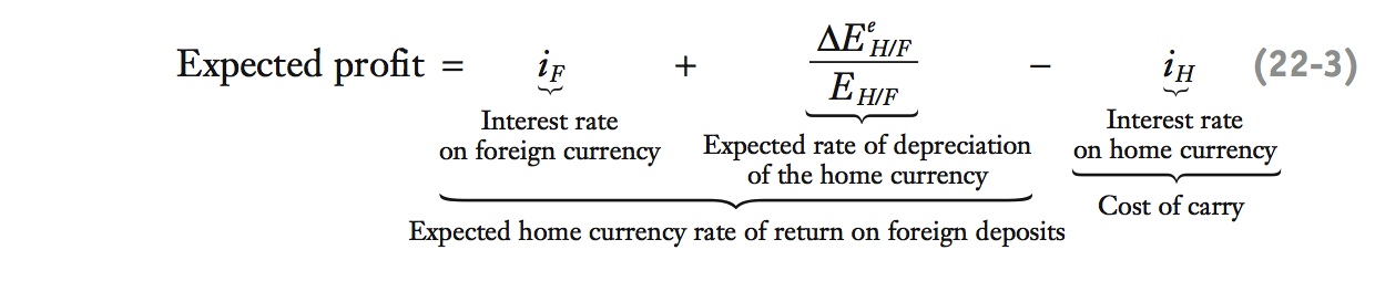
Uncovered interest parity (UIP) implies that the home interest rate should equal the foreign interest rate plus the rate of depreciation of the home currency. If UIP holds, it would seem to rule out the naive strategy of borrowing in a low interest rate currency and investing in a high interest rate currency, an investment referred to as a carry trade. In other words, UIP implies that the expected profit from such a trade is zero:
462
From the home perspective, the return to an investment in the foreign currency (the foreign return) consists of the first two terms on the right-hand side of the preceding equation. Let’s suppose the foreign currency (that of Australia, say) has a high interest rate of 6%. Now suppose the home country (Japan, say) has a low interest rate of 1%. The final term in the preceding equation is the cost of borrowing funds in local currency (Japanese yen) or, in financial jargon, the cost of carry. The interest rate differential, 5%, would be the profit on the carry trade if the exchange rate remained unchanged. If UIP is true, however, it would be pointless to engage in such arbitrage because the low-yield currency (the yen) would be expected to appreciate by 5% against the high-yield currency (the Australian dollar). The exchange rate term would be −5%, leaving zero expected profit.
The Long and Short of It In the past decade or two, the predominant low interest rate currencies in the world economy have been the Japanese yen and the Swiss franc, and carry traders have often borrowed (“gone short”) in these currencies and made an investment (“gone long”) in higher interest rate major currencies such as the U.S. dollar, pound sterling, euro, Canadian dollar, Australian dollar, and New Zealand dollar. The profits from these trades have been very large. Has UIP failed?
To grasp how a carry trade functions, Figure 22-4, panel (a), shows actual monthly profits (in percent per month) from a carry trade based on borrowing low-interest yen in the Japanese money market and investing the proceeds in a high-interest Australian dollar money market account for one month. Also shown are the cumulative profits (in yen) that would have accrued from a ¥100 carry trade initiated on January 1, 1992. Panel (b) shows the underlying data used to calculate these returns. We see that over this entire period, the annual Australian dollar interest rate exceeded the Japanese yen interest rate, often by five or six percentage points. Thus, returns would be positive for this strategy if the yen depreciated or even appreciated only slightly against the Australian dollar. But if the yen appreciated more than slightly in any month, returns would be negative, and losses would result.
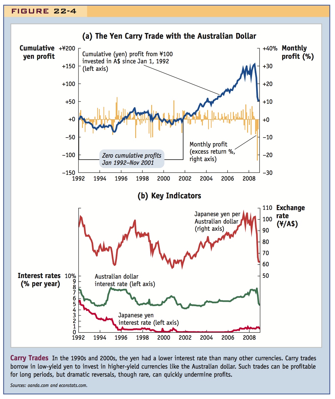
Panel (a) shows that in many months the high interest being paid on the Australian dollar was not offset by yen appreciation, and the carry trade resulted in a profit; this pattern was seen frequently in the period from 1995 to 1996, for example. There were other periods, however, when a sharp yen appreciation far exceeded the interest differential, and the carry trade resulted in a loss; this pattern occurred quite a bit in late 1998 and again during the global financial crisis of 2008. In 1998, for example, in each of three months, in fact—August, October, and December 1998—the Australian dollar lost about 10% in value, wiping out the profits from two years’ worth of interest differentials in all three cases. Overall, we see that the periods of positive and negative returns were driven not by the fairly stable interest differential seen in panel (b), but by the long and volatile swings in the exchange rate.
To sum up, the carry trade strategy was subject to a good deal of volatility, and over the decade from the start of 1992 to the end of 2001, the highs and lows canceled each other out in the long run. On November 1, 2001, for example, the average return on this carry trade was virtually zero. Cumulative interest since 1992 on the two currencies expressed in yen was virtually the same, about 13%. Over that period, 100 yen placed in either currency at the start would have been worth 113 yen by the end.
What happened after that date? Subsequent trends again caused the value of Australian investment to pull ahead, as can be seen in panel (a) by the mostly positive returns registered month after month from 2002 to 2006. By June 2007 cumulative profits were well over ¥100. The reason? As panel (b) shows, the yen persistently weakened against the Australian dollar over this five-year period (by about 6% to 7% per year), reinforcing the interest differential (about 6% to 7% also) rather than offsetting it. Adding up, from 2002 to 2006 the cumulative return on the carry trade was about 15% per year! Would that trend continue or was there to be another sudden swing resulting from yen appreciation? As we can see, another wipeout came along in 2008. This question brings us to a consideration of the role of risk in the forex market.
463
464
Investors face very real risks in this market. Suppose you put up $1,000 of your own capital and borrow $19,000 in yen from a bank. You now have 20 times your capital, a ratio, or leverage, of 20 (not uncommon). Then you play the carry trade, investing the $20,000 in the Australian dollar. It takes only a 5% loss on this trade to wipe you out: 5% of $20,000 eats all your capital. And without that margin to back you up, the bank bids you goodbye. As we have seen, losing 5% in a month is quite possible, as is losing 10% or even 15%.
For policy makers and market participants, the broader fear is that while big losses for households would be bad enough, big losses at large, high-leverage financial institutions could have damaging spillover effects in the global macroeconomy. For example, in June 2007, Jim O’Neill, Goldman Sachs chief global economist, said investment firms had been caught on the wrong side of huge bets against the Japanese yen: “There has been an amazing amount of leverage on currency markets that has nothing to do with real economic activity. I think there are going to be dead bodies around when this is over. The yen carry trade has reached 5% of Japan’s GDP. This is enormous and highly risky, as we are now seeing.”7 Days later Steven Pearson, chief currency strategist at HBOS bank, said, “A sizeable reversal at some point is highly likely, but the problem with that statement is the ‘at some point’ bit, because carry trades make money steadily over long periods of time.”8
In the carry trade, as history shows, a big reversal can always happen as everyone rushes to exit the carry trades and they all “unwind” their positions at the same time. The answer to the dangling question above is yes, a big reversal did come along for the trade in question: after rising another 10% against the yen from January to July 2007, the Australian dollar then fell by 15% in the space of a month, eating up about three years’ worth of interest differential for anyone unlucky enough to buy in at the peak. Many hedge funds and individual investors who made ill-timed or excessively leveraged bets lost a bundle (see Headlines: Mrs. Watanabe’s Hedge Fund).
Still, given the persistence of profits, anyone predicting such reversals may appear to be crying wolf. Money managers often face incentives to follow the herd and the market’s momentum keeps the profits flowing—until they stop. All this ensures high levels of stress and uncertainty for anyone in the forex trading world and for some of the households engaged in this kind of risky arbitrage.
Carry Trade Summary Our study of the carry trade focuses our attention on several facts. First, even if expected returns from arbitrage are zero, actual realized returns are often not zero. Second, such returns appear to be persistent. Third, the returns are also very volatile, or risky. All of these issues need to be addressed as we judge the success or failure of UIP.
Have students look at Figure 22-4. Emphasize that carry profits are very volatile, and can often go very negative.
Three important stylized facts.
The expected returns from arbitrage may also be non-zero under fixed rates. If there are expectations of depreciation, interest rates won’t equalize. Hong Kong during the 1997 crisis is an example of a depreciation that was expected but that did not occur. But the carry trade earned positive returns during the crisis. Argentina in 2000-2001 is an example of a depreciation that was expected and did occur. The carry trade earned negative returns. The fact that expectations may not be realized, even under fixed rates, is called the peso problem. The failure of UIP ex post, however, is arguably not a sign of irrationality, but merely a reflection of the fact that people had rational expectations of a depreciation that did not actually come to pass.
Peso Problems
The example of carry trades between the Japanese yen and the Australian dollar shows how actual returns from interest arbitrage may be nonzero (but risky) for a pair of currencies that are floating. But the same can be true for two currencies that are fixed. To illustrate this case, we turn to recent data involving the U.S. dollar pegs of two emerging market countries, Hong Kong and Argentina.
465
The carry trade is now undertaken not only by large financial institutions, but also increasingly by individual Japanese investors.
Mrs. Watanabe’s Hedge Fund
The OECD estimated the total yen carry trade at $4 trillion in 2006. This trade involves not just large financial institutions but increasing numbers of Japanese individual investors, who place money in high-yielding foreign currency deposits or uridashi bonds.
TOKYO—Since the credit crisis started shaking the world financial markets this summer, many professional traders have taken big losses. Another, less likely group of investors has, too: middle-class Japanese homemakers who moonlight as amateur currency speculators.
Ms. Itoh is one of them. Ms. Itoh, a homemaker in the central city of Nagoya, did not want her full name used because her husband still does not know. After cleaning the dinner dishes, she would spend her evenings buying and selling British pounds and Australian dollars.
When the turmoil struck the currency markets last month, Ms. Itoh spent a sleepless week as market losses wiped out her holdings. She lost nearly all her family’s $100,000 in savings.
“I wanted to add to our savings, but instead I got in over my head,” Ms. Itoh, 36, said.
Tens of thousands of married Japanese women ventured into online currency trading in the last year and a half, playing the markets between household chores or after tucking the children into bed. While the overwhelmingly male world of traders and investors here mocked them as kimono-clad “Mrs. Watanabes,” these women collectively emerged as a powerful force, using Japan’s vast wealth to sway prices and confound economists….
Now Japan’s homemaker-traders may become yet another casualty of the shakeout hitting the debt, credit and stock markets worldwide…. Most analysts estimate that Japanese online investors lost $2.5 billion trading currency last month….
Some of the women used their own money, some used their husband’s, and some used a combination of both. But by trading, they challenged deeply held social prohibitions in Japan against money, which is often seen here as dirty, especially when earned through market speculation.
“There are strict taboos against money that isn’t earned with sweat from the brow,” said Mayumi Torii, a 41-year-old mother of one who said she earned $150,000 since she started margin trading in currencies early last year.
Ms. Torii is one of Japan’s most famous housewife-traders. She has written a book on her investing strategies and founded a support group for home traders, the FX Beauties Club, which now has 40 members. (FX is financial shorthand for “foreign exchange.”)…
One reason Japan’s homemakers can move markets is that they hold the purse strings of the nation’s $12.5 trillion in household savings. For more than a decade, that money languished in banks here at low interest rates. But as the rapid aging of Japan’s population has brought anxiety about the future, households are starting to move more of it overseas in search of higher returns.
A tiny fraction of this has flowed into risky investments like online currency accounts. Most of these accounts involve margin trading, in which investors place a cash deposit with a brokerage that allows them to borrow up to 20 or even 100 times their holdings for trading.
The practice has been popular not only because it vastly raises the level of potential profits, but also because it allowed wives to trade at home, said Hiroshi Takao, chief operating officer of TokyoForex, an online trading firm.

The housewife-traders were so secretive that many market analysts did not realize how widespread the trend had become until this summer, when the police arrested a Tokyo housewife accused of failing to pay $1.1 million in taxes on her foreign exchange earnings….
For a time, margin trading seemed like a surefire way to make money, as the yen moved only downward against the dollar and other currencies. But last month, in the midst of the credit turmoil, the yen soared as hedge funds and traders panicked.
Ms. Itoh recalled that she had wanted to cry as she watched the yen jump as much as 5 percent in value in a single day, Aug. 16.
“But I had to keep a poker face, because my husband was sitting behind me,” Ms. Itoh said.
She did not sell her position, thinking the yen would fall again. But by the next morning, only $1,000 remained in her account, she said….
[M]ost of the half dozen homemaker-traders interviewed for this article said they were already trading again, and the rest said they soon would be—including Ms. Itoh, who said she would probably invest her remaining $1,000 in savings.
“There’s no other way to make money so quickly,” she said.
Source: Excerpted from Martin Fackler, “Japanese Housewives Sweat in Secret as Markets Reel,” New York Times, September 16, 2007. © 2007 The New York Times. All rights reserved. Used by permission and protected by the Copyright Laws of the United States. The printing, copying, redistribution, or retransmission of this Content without express written permission is prohibited.
466
As we saw in the chapter on fixed and floating regimes, in the case of a credibly fixed peg with no risk of a depreciation or any other risks (no currency premium and no default risk premium), the UIP condition states that the home interest rate should equal the foreign interest rate because investors treat domestic and foreign currency as perfect substitutes that always have been and always will be interchangeable at a fixed rate. Thus, the interest differential between the two currencies should be zero. Again, if true, this outcome would seem to rule out any desire on the part of investors to engage in arbitrage (e.g., via the carry trade). But there is an important exception: when pegs are not credible, risk premiums can cause large interest differentials—and cause investors to smell a profit.
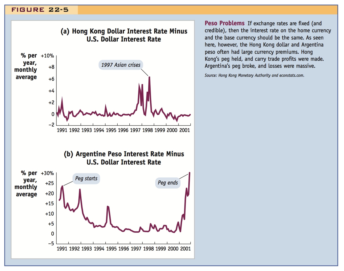
Figure 22-5, panel (a), shows data for Hong Kong from 1990 to 2001, including the crucial period in 1997 when many Asian countries were in crisis and their exchange rate pegs were breaking. Most of the time, the interest differential between the Hong Kong dollar and the U.S. dollar was zero, as one would expect for what was perceived to be a credible peg. Hong Kong was operating a quasi-currency board with reserves of approximately 300% of the (base) money supply. Short of dollarization, this was considered about the most bulletproof peg around.
467
Nonetheless, in late 1997 investors started to fear that Hong Kong might suffer the same fate as other Asian economies. Expecting a future depreciation of the Hong Kong dollar, they started to demand a currency premium. At its peak, the Hong Kong interest rate rose almost 20 percentage points per year above the U.S. interest rate in late October, and the spread exceeded 5 percentage points for over three weeks.. However, the expected depreciation never happened. The Hong Kong dollar’s peg to the U.S. dollar survived. Investors may have been reasonable to fear a crisis and demand a premium beforehand (ex ante), but after the fact (ex post), these unrealized expectations became realized profits. As a result, there was a lot of money to be made from the carry trade for those willing to park their money in Hong Kong dollars during all the fuss.
Should you always bet on a peg to hold in a crisis? No. Figure 22-5, panel (b), shows data for Argentina from 1991 to 2001. This includes the period of looming crisis for the Argentine economy in 2001, as the likelihood of default and depreciation grew. The country was in fiscal trouble with an ailing banking sector. It no longer had the ability to borrow in world capital markets and was about to be cut off from International Monetary Fund assistance. A recession was deepening. All of this was raising the pressure on the government to use monetary policy for purposes other than maintaining the peg. Investors began to demand a huge currency-plus-default premium on Argentine peso deposits to compensate them for the risk of a possible depreciation and/or banking crisis. Peso interest rates at one point were more than 25% above the U.S. interest rate. But in this case, investors’ fears were justified: in December 2000 to January 2001 the Argentine government froze bank deposits, imposed capital controls, and the peg broke. The peso’s value plummeted, and soon the exchange rate exceeded three pesos to the dollar, erasing more than two-thirds of the U.S. dollar value of peso deposits. In retrospect, the precrisis interest differentials had been too small: the carry traders who gambled and left their money in peso deposits eventually lost their shirts.
Possibly digress to explain the origin of the term: The Mexican peso was pegged to the U.S., but sold at a persistent forward premium. Ex ante there was a small probability of a regime change, for which investors required compensation. Ex post though, the regime change didn't occur, so if you just look at ex post data you might think people were persistently mistaken about their beliefs.
We can now see how expectations may not be realized, even when exchange rates are fixed. Fixed exchange rates often break, and investors may reasonably demand currency premiums at certain times. However, after the fact, such premiums may lead to returns from interest arbitrage that are positive (when pegs hold, as in the Hong Kong case) or negative (when pegs break, as in the Argentine case).

International economists refer to this phenomenon as the peso problem (given its common occurrence in a certain region of the world). But again, it is far from clear that the profits seen are a sign that UIP fails or that investors are acting irrationally. The collapse of a peg can be seen as a rare event, an extreme occurrence that is hard to predict but that will lead to large changes in the values of assets. This situation is not unlike, say, fire or earthquake insurance: every year that you pay the premium and nothing happens, you make a “loss” on the insurance arrangement, a pattern that could go on for years (hopefully, for your entire life), but you know that the insurance will pay off to your advantage in a big way if disaster strikes.
468
The Efficient Markets Hypothesis
1. The Efficient Markets Hypothesis
Write actual (or ex post) profit as i - i* + ΔE⁄E = 0; . The forecast error is then the difference between actual and expected profit, which is just ΔE⁄E - ΔEe⁄E What do unexpected profits tell us about UIP?
a. Expected Profits
Use survey data to measure traders expected profits. Plot them against the interest differential. If UIP holds, the expectations should be on the 45-degree line. Ex ante UIP seems to do pretty well.
b. Actual Profits
Now plot actual profits against the interest differential. There are plenty of unanticipated profits and losses. Furthermore, the line of best fit has a slope of .2. This means that for every 1 percent interest differential we should expect only a .2 percent appreciation—implying a profit of .8.
c. The UIP Puzzle
The fact that the line of best fit is below 1 means that when the interest differential is high actual depreciation is usually less than anticipated. This implies that the carry trade is profitable. This is anomalous because it means people don’t have rational expectations, the idea that, on average, actual and expected values should be the same. It also violates the efficient markets hypothesis, which asserts that asset prices should reflect all currently available information. The UIP Puzzle: Why are there predictable profits in the carry trade?
2. Limits to Arbitrage
How to explain the puzzle? As with PPP, invoke trade costs
a. Trade Costs Are Small
Trading costs in financial markets too small to explain the puzzle
b. Risk Versus Reward
Return to the plot of returns against the interest differential. Imagine a carry strategy of borrowing from the low interest country to lend in the high interest country. The fact that the line of best fit is flatter than the 45-degree line we should expect to make a profit. Two problems with this strategy: (1) Profits do not grow linearly with the interest differential; the linear model doesn’t predict well. (2) Profits are very volatile, or risky.
c. The Sharpe Ratio and Puzzles in Finance
Carry trade profit is an example of an excess of returns, the difference between a risky return and a riskless return. The Sharpe ratio of an asset is defined as the ratio of its mean excess return to its standard deviation: It measures how much investors are rewarded with expected returns from the asset to compensate them from taking on its risk. Sharpe ratios for the carry trade are around .5. Based upon stock market returns, where the Sharpe ratio is about .48, many investors would consider this too small. There are excess returns in the stock market but, given conventional measures of risk aversion, it is hard to explain why people don’t arbitrage the stock market more. Behavioral finance may have some answers (loss aversion or limited rationality, for example). In the FX data the Sharpe ratio is close to that in the stock market. Perhaps the ratio of reward to risk is so small that people have no interest in arbitraging.
d. Predictability and Nonlinearity
Nonlinear models predict that profits should be low at both low and high interest differentials. Sharpe ratios are positive only in the middle-range on interest differentials. Perhaps nonlinear strategies should make investment depend more upon the magnitude of the expected return. But the Sharpe ratios would still be quite low.
3. Conclusion
There seem to be predictable excess returns on the FX market. However the Sharpe ratio is too low to attract more investors. Arbitrage probably hasn’t failed, it has just gone about as far as can be expected. There is no evidence of vast, unexploited profits on the FX market. Importance: the limits to arbitrage may allow deviations from UIP in some cases.
Make sure students understand the difference.
Do carry trade profits disprove UIP? To explore this question further, let us rewrite Equation (11-3), which calculates expected profits, by replacing expected or ex ante values of the exchange rate with actual or ex post realized values.
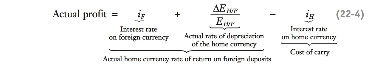
Note the one subtle difference: the disappearance of the superscript “e,” which denoted expectations of future exchange rate depreciation. This expression can be computed only after the fact: although interest rates are known in advance, the future exchange rate is not. We know actual profits only after the investment strategy has run its course.
Thus, the sole difference between actual and expected profits is a forecast error that corresponds to the difference between actual depreciation and expected depreciation. (Again, the importance of exchange rate forecasts is revealed!) This forecast error is the difference between Equation (11-3) and Equation (11-4), that is,

Emphasize that UIP is an ex ante hypothesis.
Armed with this way of understanding unexpected profits, we can now confront an important and controversial puzzle in international macroeconomics: What can the behavior of this forecast error tell us about UIP and the workings of the forex market? One way to attack that question is to study expected and actual profits side by side to see the size of the forecast error and its pattern of behavior.
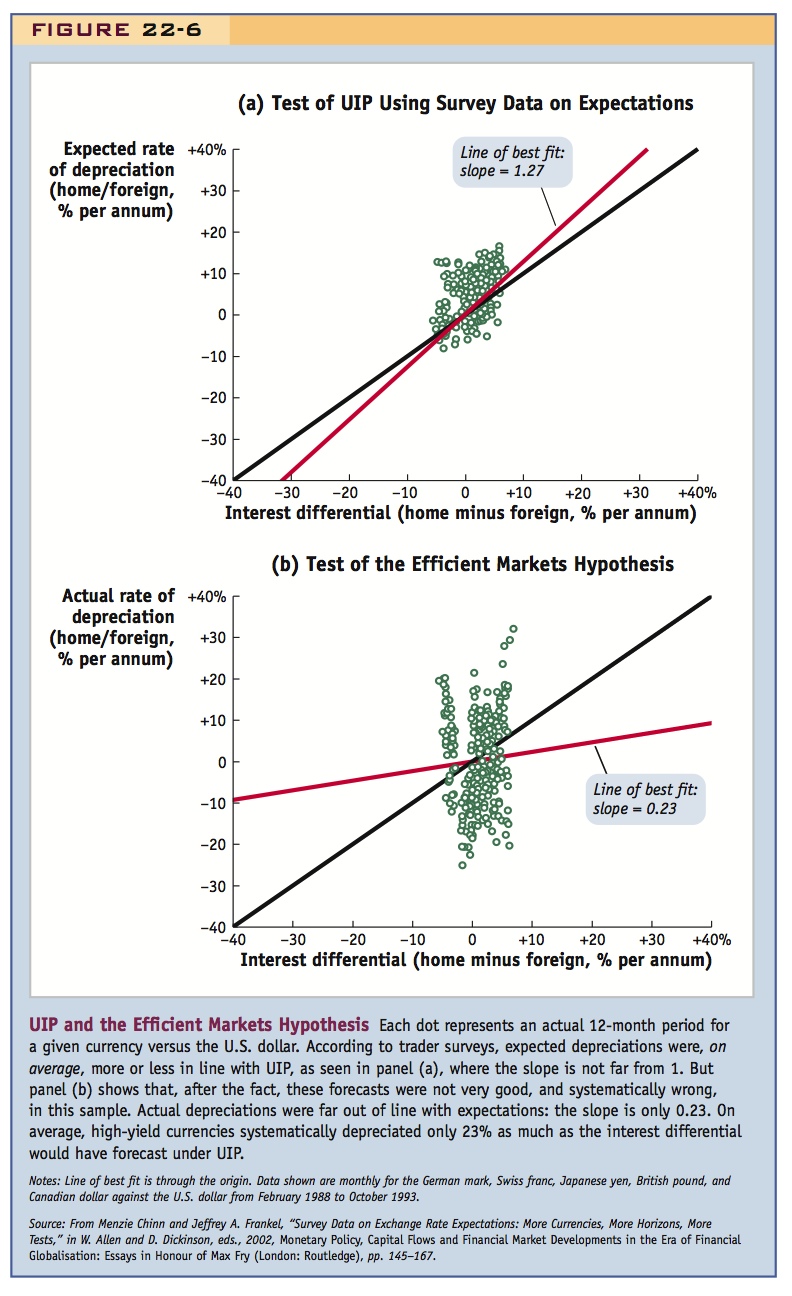
Expected Profits On the one hand, strictly speaking, UIP itself says nothing about the forecast error. It says only that before that fact, or ex ante, expected profits should be zero. Expectations are not directly observable in markets, but we can recall the evidence presented in the chapter on exchange rates in the short run based on surveys of traders’ expectations for major currencies from 1988 to 1993. As a recap, Figure 22-6, panel (a), presents this evidence again. The figure plots the expected depreciation against the interest differential for several major currencies.9
Assert the stylized fact that on average expected profits are in fact zero.
On the 45-degree line, these two terms are equal, and expected profits will be zero, according to Equation (11-3). As in several studies of this sort, on average, the data are aligned close to, but not exactly on, the 45-degree line, so they are not wildly inconsistent with UIP. The line-of-best-fit slope is close to 1. But the survey data are probably prone to error and cover only some (but not all) of the traders in the market. Even using formal statistical tests, it is difficult to reject UIP based on shaky evidence of this sort. The hypothesis that UIP holds can typically survive this kind of test.
Actual Profits On the other hand, we know that actual profits are made. It is enlightening to see exactly how they are made by replacing the expected depreciation in panel (a) with actual depreciation, after the fact, or ex post. This change is made in panel (b), which, to be consistent, shows actual profits for the same currencies over the same period.
469
470
The change is dramatic. There are plenty of observations not on the 45-degree line, indicating that profits and losses were made in some periods. Even more striking, the line of best fit has a slope of about 0.2. This means that for every 1% of interest differential in favor of the foreign currency, we would expect only a 0.2% appreciation of the home currency, on average, leaving a profit of 0.8%. At larger interest differentials, the line of best fit means even larger profits. (Some studies find zero, or even negative slopes, implying even bigger profits!)
And yet on average there are forecastable profits from the carry trade.
The UIP Puzzle A finding that profits can be made needs careful handling. On its own, this need not imply a violation of UIP: random profits could arise due to variation about a zero mean. However, looking at actual profits, the pattern of the deviations from the 45-degree line is systematic. The slope of the best-fit line is well below 1, indicating, for example, that when the interest differential is high, actual depreciation is typically less than expected and less than the interest differential. In other words, on average, the carry trade (borrowing in the low-yield currency to invest in the high-yield currency) is profitable. Actual profits are risky, but they appear to be forecastable.
This might seem cryptic to students who have never encountered this idea before. It might require more explanation. Suggestion: Use stock prices as a motivating example. Expected profits are Ep(t+1) - p(t). Explain why arbitrage requires this to equal zero, absent a risk premium. Then define rational expectations: p(t+1) = Ep(t+1) + u(t+1), with Eu(t+1) = 0 and uncorrelated with time t info. Given arbitrage and rational expectations derive the random walk (efficient market) hypothesis, p(t+1) = p(t) + u(t+1). Conclude that on average you can't beat the market.
This finding is widely considered to be a puzzle or anomaly. If such profits are forecastable, then the forex market would be violating some of the fundamental tenets of the modern theory of finance. The rational expectations hypothesis argues that, on average, all investors should make forecasts about the future that are without bias: on average, actual and expected values should correspond. But, as we just saw, the difference between actual and expected exchange rates reveals a clear bias.
Next apply the same reasoning to FX. Use rational expectations and 22-3 (UIP) to show that the actual rate of depreciation should equal the interest differential (= forward premium) plus an unpredictable error term if the FX market is efficient.
In addition, the efficient markets hypothesis, developed by economist Eugene Fama, asserts that financial markets are “informationally efficient” in that all prices reflect all known information at any given time. Hence, such information should not be useful in forecasting future profits: that is, one should not be able to systematically beat the market.
Fama emphasizes that the EMH is always a joint hypothesis of rational expectations and a specific data generating mechanism (a model). For example, if people are risk averse then there could be a systematic deviation from UIP even if people are rational.
Ultimately then, the UIP puzzle isn’t just about UIP. The expectations data (the best that we have) suggest that UIP does hold. The real UIP puzzle is why UIP combined with the rational expectations and efficient markets hypotheses fails to hold. Yet these hypotheses seemingly do fail. This appears to be an inefficient market instead. Why are those big forecastable profits lying around?
Limits to Arbitrage
This is a nice way to link up this section on UIP with the previous on PPP, but trading costs are inconsequential here.
Economists have proposed a number of ways to resolve these puzzles, and at some level all of these can be described as explanations based on a limits to arbitrage argument. What does this mean? In the first section of this chapter, we argued that there were limits to arbitrage, in the form of trade costs, that can help explain the PPP puzzle: purchasing power parity will not hold if there are frictions such as transport costs, tariffs, and so on that hamper arbitrage in goods markets.
Limits to arbitrage arguments can also be applied in the world of finance. But how? And can they help explain the UIP puzzle?
Trade Costs Are Small It is tempting but ultimately not fruitful to look for the same kinds of frictions that we saw in goods markets. Conventional trade costs in financial markets are simply too small to have an effect that is large enough to explain the puzzle. There are bid-ask spreads between currencies, and there may be other technical trading costs, for example, associated with when a forex trade is placed during the day and which financial markets are open. But none of these frictions provides a sufficient explanation for the forecastable profits and the market’s inefficiency.
471
There is also the problem that if one wishes to make a very large transaction, especially in a less liquid currency, the act of trading itself may have an adverse impact on the exchange rate and curtail profitable trades. For example, an order for $1 billion of more liquid yen is more easily digested by the market than an order for $1 billion of less liquid New Zealand dollars. But again, this possibility is not likely to explain the UIP puzzle because investors can avert such a situation by breaking their trades up into small pieces and spreading them out over time. So even though these trading costs are real, they may not be large enough to offset the very substantial profits we have seen.
If trading costs are the sole limit to arbitrage, there is still a puzzle. We must look elsewhere.
Risk Versus Reward A promising approach to the puzzle examines traders’ alternative investment strategies, draws on other puzzles in finance, is based less on introspection and more on observations of actual trading strategies, and connects with the frontiers of the emerging field of behavioral economics.
To approach this research and to make the investment problem facing the trader a little clearer, we can reconsider the data shown in Figure 22-6. In panel (b) we saw that the slope was only 0.23, meaning that for every 1% of interest differential, we would predict only 0.23% of offsetting depreciation, leaving a seemingly predictable profit of 0.77%. Suppose we followed a carry trade strategy of borrowing in the low interest rate currency and investing in the high-interest currency. If the interest differential were 1%, then we would expect to net a profit of 0.77%; if the interest differential were 2%, we would expect to double that profit to 1.54%; a differential of 3% would yield 2.31% profit, and so on, if we simply extrapolate that straight line.
This strategy would have delivered profits. However, there are two problems with it. First, profits do not, in fact, grow linearly with the interest differential. The straight-line model is a poor fit. At high-interest differentials there are times when profits are very good, and other times when the carry trade suffers a reversal, and large losses accrue, as we have seen. The second problem is a related one. At all levels of the interest differential, Figure 22-6 clearly shows the extreme volatility or riskiness of these returns due to the extreme and unpredictable volatility of the exchange rate. Actual rates of depreciation can easily range between plus or minus 10% per year, and up to plus or minus 30% in some cases.
One measure of the volatility of returns used by economists is the standard deviation, which we can now put to use to explore why these positive but risky profits are left unexploited.
The Sharpe Ratio and Puzzles in Finance Carry trade profits are the difference between a risky foreign return and a safe domestic interest rate. This kind of return difference is called an excess return, and to analyze it further, we can draw on one of the standard tools of financial economics.
The Sharpe ratio is the ratio of an asset’s average annualized excess return to the annualized standard deviation of its return:

472
The ratio was invented by William Forsyth Sharpe, a Nobel laureate in economics. As a ratio of “rewards to variability,” the Sharpe ratio tells us how much the returns on an asset compensate investors for the risks they take when investing in it.
Figure 22-7 displays data on returns to the simple carry trade strategy for several major currencies against the British pound for the period 1976 to 2005. For each pair of currencies, it is assumed that each month a trader would have borrowed in the low interest rate currency and invested in the high interest rate currency. Details on the returns to a portfolio of all such trades (equally weighted) are also shown.
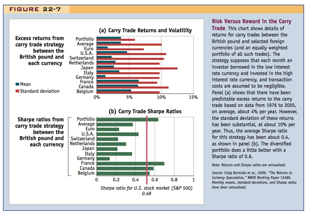
In panel (a) we see that the returns to these strategies were positive for all currencies (they were also statistically significant), and, on average, they were about 4% per year. However, the volatility of the returns was even larger in all cases, as measured by the standard deviation. On average, this was about 10% on an annual basis, although falling to 6% for the portfolio (due to gains from diversification). In panel (b) the corresponding Sharpe ratios are shown, and we can see that they fall below 1 in all cases. The average for all currencies is 0.4 and, thanks to a reduction in volatility due to diversification, the equally weighted portfolio has a modestly higher Sharpe ratio of 0.6.
We now must ask: Should Sharpe ratios of around 0.5 be considered “big” or “small”? Do they signal that investors are missing a profit opportunity? Should people be rushing to take profits in investments that offer this mix of risk and reward? If this can be judged to be a “big” Sharpe ratio, then we have a puzzle as the market would seem to be failing in terms of efficiency.
473
Relate this to risk aversion?
It turns out that many investors in the forex market would consider that 0.5 is a fairly small Sharpe ratio. To see why, and to understand how this approach may “solve” the UIP puzzle, we note that historically, as shown in panel (b), the annual Sharpe ratio for the U.S. stock market has been about 0.48, based on the excess returns of the broad S&P 500 index over and above risk-free U.S. Treasury bonds. This reference level of 0.48 might be thought of as a hurdle that competing investment strategies must beat if they are to attract additional investment. But we can see from panel (b) that forex carry trades either fall below this bar, or just barely surmount it.
This may also require some explanation.
There are indeed excess returns in the stock market, but investors are not rushing to borrow money to buy stocks to push that Sharpe ratio any lower. Admittedly, many economists consider the stock market finding to be a puzzle (called the equity premium puzzle) because under various standard theories and assumptions about risk aversion, it is hard to understand why investors sit back and leave such excess returns on the table. And yet they do, a fact that leads other economists to postulate that some very nonstandard assumptions, some drawn from psychology, may now need to be included in models to properly explain investor behavior. Research in behavioral finance, a branch of behavioral economics, attempts to explain such seemingly irrational market outcomes using various principles such as rational action under different preferences (e.g., strong aversion to loss) or more limited forms of rationality (e.g., models with slow or costly learning).
To sum up, there are now theories that might explain why nobody arbitrages the stock market when its Sharpe ratio is 0.48. That just isn’t a high enough reward-risk ratio to attract investors. But in our forex market data, the Sharpe ratio is about the same, and most other studies find carry trade Sharpe ratios that are little larger than the stock market’s 0.48.10 So we may have an answer to the question why arbitrage does not erase all excess returns. The ratio of rewards to risk is so very small that investors in the market are simply uninterested. Indeed, surveys of trader behavior in major firms by economist Richard Lyons suggest that, in the forex market, if the predicted Sharpe ratio of a strategy falls below even 1, then this is enough to discourage investor interest.11
Predictability and Nonlinearity Can we do better than a straight-line model or linear predictions of returns and crude carry trade strategies? More complex and diversified forex trading strategies may be able to jack up the Sharpe ratio a little, but not too much. As an alternative way of describing the data, for example, we can use nonlinear models that fit the data quite well.12
Nonlinear models show that at low interest differentials (say, 0% to 2%), profits are inherently low, and nobody has been much interested in arbitrage given the risks; conversely, at high differentials (say, 5% or more), the rewards have often vanished as investors have rushed in, bid up the high-yield currency to its maximum value, causing a reversal that wipes out carry trade profits. At the extremes, arbitrage has tended to work when it should (or shouldn’t). Only in the middle do moderate, positive Sharpe ratios emerge, it seems, for investors willing to take some risks. Thus, our “small” average Sharpe ratios are a mix of these low and high returns, suggesting more sophisticated strategies should ensure that the investment decision depends on the size of the expected return. But the rewards relative to risk are still quite meager and Sharpe ratios are still fairly low even when arbitrage looks most promising.
474
Conclusion
The main lesson here is that risky arbitrage is fundamentally different from riskless arbitrage. Based on this sort of standard financial analysis, many economists conclude that although there may be excess returns, even predictable excess returns, in the forex market, the risk-reward ratio is typically too low to attract additional investors.13 In that sense, there is no puzzle left and arbitrage has not failed—it has just gone as far as might be reasonably expected, at least given investor behavior in equity markets and elsewhere. In forex market research, nobody has yet proved that there are large amounts of low-risk money lying on the table (though if they did, they might not publish the result).
What are the implications? Here, there is common ground between the UIP and PPP puzzles. In the case of the PPP puzzle studied earlier in the chapter, limits to arbitrage in the goods market (mainly due to transaction costs) may create a band of inaction allowing for deviations from parity in purchasing prices. In the case of the UIP puzzle, limits to arbitrage in the forex market (mainly due to risk) may allow for deviations from interest parity in some situations.