1 Movement of Labor Between Countries: Migration
1. Objective: Analyze the effects on factor returns of migration from Foreign to Home, given world relative prices of goods.
We begin with the examples of labor migration described by the Mariel boat lift and the Russian migration to Israel. We can think of each migration as a movement of labor from the Foreign country to the Home country. What is the impact of this movement of labor on wages paid at Home? To answer this question, we make use of our work in Chapter 3, in which we studied how the wages paid to labor and the rentals paid to capital and land are determined by the prices of the goods produced. The prices of goods themselves are determined by supply and demand in world markets. In the analysis that follows, we treat the prices of goods as fixed and ask how the Home wage and the rentals paid to capital and land change as labor moves between countries.
Effects of Immigration in the Short Run: Specific-Factors Model
2. Effects of Immigration in the Short Run: Specific-Factors Model
a. Determining the Wage
As in Chapter 3, the wage is determined by the equality of VMPLs in the two sectors, given the endowment of labor.
b. Effect of Immigration on the Wage in Home
Migration from Foreign stretches the graph to the right, pulling VMPLA to the right. Wages fall. Conclusion: In the specific-factors model, migration from Foreign will lower the wage at Home.
We begin our study of the effect of factor movements between countries by using the specific-factors model we learned in Chapter 3 to analyze the short run, when labor is mobile among Home industries, but land and capital are fixed. After that, we consider the long run, when all factors are mobile among industries at Home.
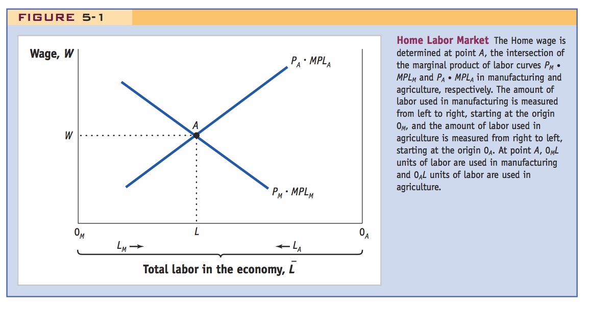
Determining the Wage Figure 5-1 shows a diagram that we used in Chapter 3 to determine the equilibrium wage paid to labor. The horizontal axis measures the total amount of labor in the economy  , which consists of the labor used in manufacturing LM and the amount used in agriculture LA:
LM + LA =
126
In Figure 5-1, the amount of labor used in manufacturing LM is measured from left (0M) to right, and the amount of labor used in agriculture LA is measured from right (0A) to left.
Believe it not, students sometimes stumble on this too: they don't see why one VMPL curve is positively sloped! Explain carefully what is being measured on the horizontal axis; draw the VMPLA in its "normal" incarnation and ask them to visualize it being physically picked up and turned around.
The two curves in Figure 5-1 take the marginal product of labor in each sector and multiply it by the price (PM or PA) in that sector. The graph of PM · MPLM is downward-sloping because as more labor is used in manufacturing, the marginal product of labor in that industry declines, and wages fall. The graph of PA · MPLA for agriculture is upward-sloping because we are measuring the labor used in agriculture LA from right to left in the diagram: as more labor is used in agriculture (moving from right to left), the marginal product of labor in agriculture falls, and wages fall.
The equilibrium wage is at point A, the intersection of the marginal product curves PM · MPLM and PA · MPLA in Figure 5-1. At this point, 0ML units of labor are used in manufacturing, and firms in that industry are willing to pay the wage W = PM · MPLM. In addition, 0AL units of labor are used in agriculture, and farmers are willing to pay the wage W = PA · MPLA. Because wages are equal in the two sectors, there is no reason for labor to move between them, and the Home labor market is in equilibrium.
In the Foreign country, a similar diagram applies. We do not draw this but assume that the equilibrium wage abroad W* is less than W in Home. This assumption would apply to the Cuban refugees, for example, who moved to Miami and to the Russian emigrants who moved to Israel to earn higher wages as well as to enjoy more freedom. As a result of this difference in wages, workers from Foreign would want to immigrate to Home and the Home workforce would increase by an amount ΔL, reflecting the number of immigrants.
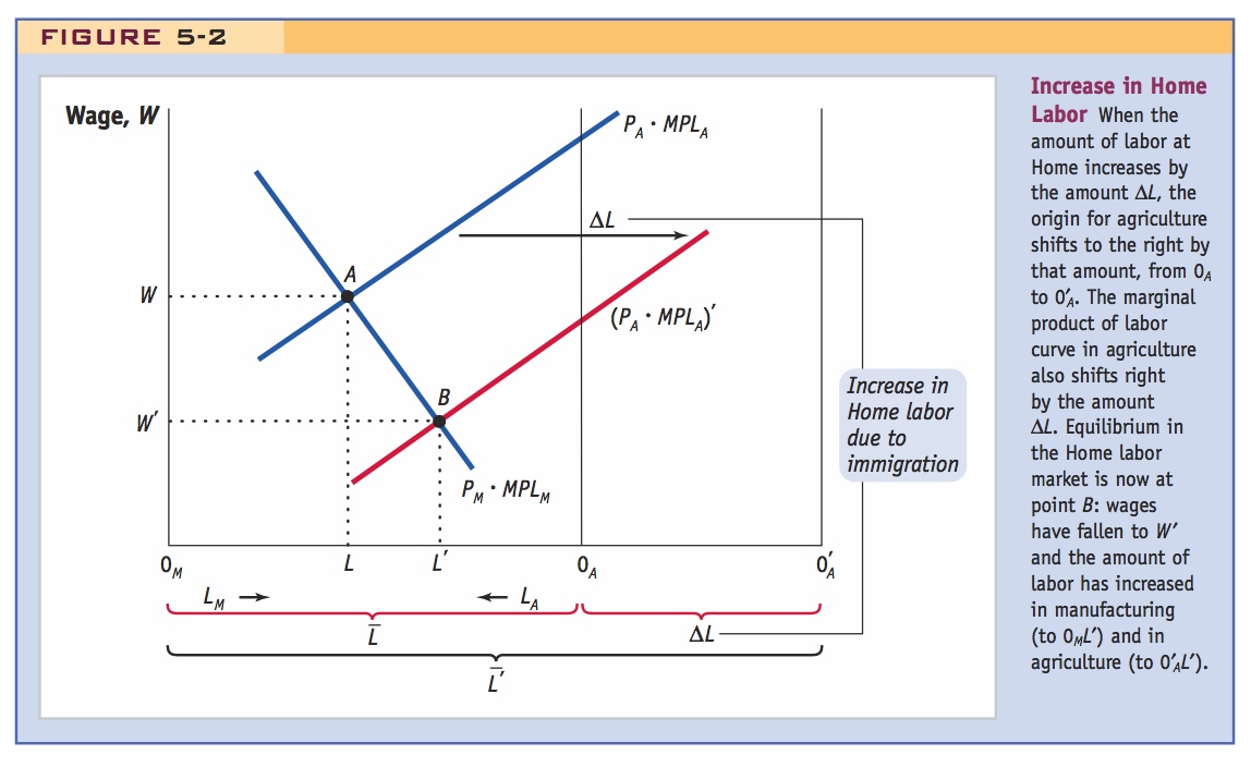
Effect of Immigration on the Wage in Home The effects of immigration are shown in Figure 5-2. Because the number of workers at Home has grown by ΔL, we expand the size of the horizontal axis from to  . The right-most point on the horizontal axis, which is the origin 0A for the agriculture industry, shifts to the right by the amount ΔL. As this origin moves rightward, it carries along with it the marginal product curve PA · MPLA for the agriculture industry (because the marginal product of labor curve is graphed relative to its origin). That curve shifts to the right by exactly the amount ΔL, the increase in the Home workforce. There is no shift in the marginal product curve PM · MPLM for the manufacturing industry because the origin 0M for manufacturing has not changed.4
127
The new equilibrium Home wage is at point B, the intersection of the marginal product curves. At the new equilibrium, the wage is lower. Notice that the extra workers ΔL arriving at Home are shared between the agriculture and manufacturing industries: the number of workers employed in manufacturing is now 0ML′, which is higher than 0ML, and the number of workers employed in agriculture is  , which is also higher than 0AL.5 Because both industries have more workers but fixed amounts of capital and land, the wage in both industries declines due to the diminishing marginal product of labor.
Emphasize this punchline.
We see, then, that the specific-factors model predicts that an inflow of labor will lower wages in the country in which the workers are arriving. This prediction has been confirmed in numerous episodes of large-scale immigration, as described in the applications that follow.
128
This is a great example to start with because it won't provoke much debate.
Massive immigration from Europe to the New World from 1870 to 1913: In 1913 real wages were higher in both Europe and the New World than in 1870. This was due to capital accumulation. However wages grew more slowly in the New World.
Immigration to the New World
Between 1870 and 1913, some 30 million Europeans left their homes in the “Old World” to immigrate to the “New World” of North and South America and Australia. The population of Argentina rose by 60% because of immigration, and Australia and Canada gained 30% more people. The population of the United States increased by 17% as a result of immigration (and it absorbed the largest number of people, more than 15 million). The migrants left the Old World for the opportunities present in the New and, most important, for the higher real wages. In Figure 5-3, we show an index of average real wages in European countries and in the New World (an average of the United States, Canada, and Australia).6 In 1870 real wages were nearly three times higher in the New World than in Europe—120 as compared with 40.
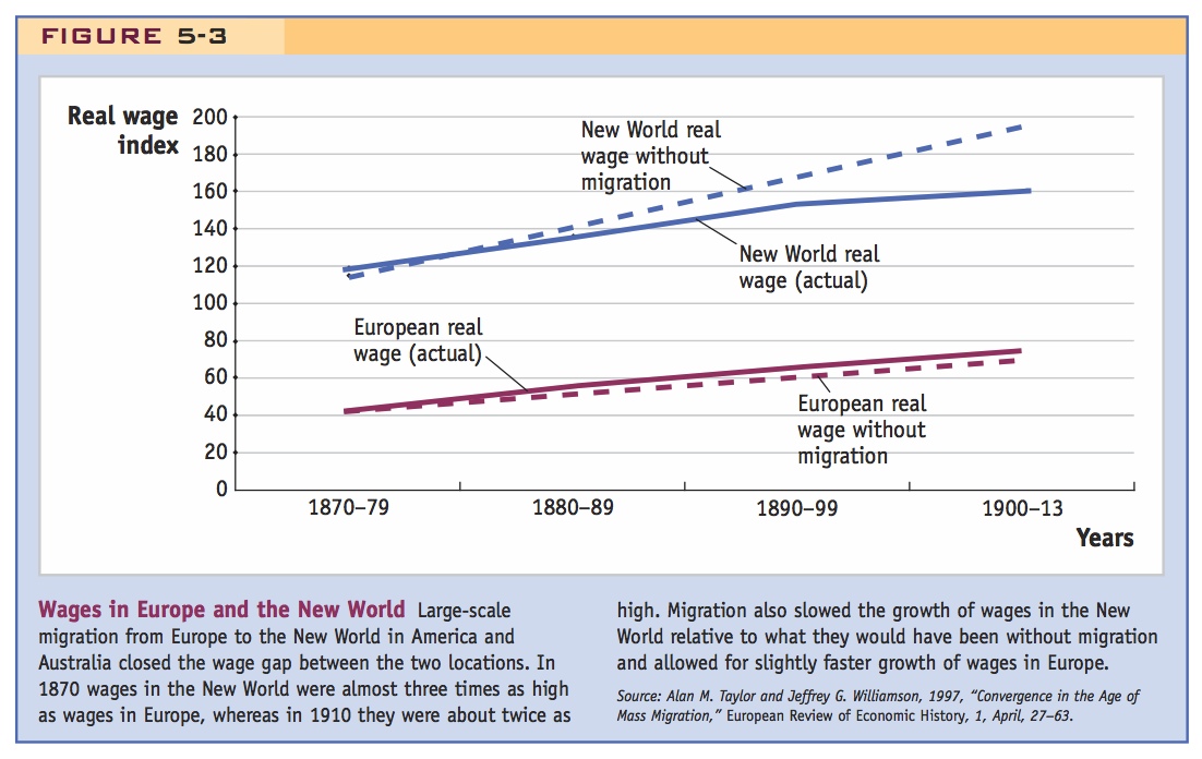
Real wages in both locations grew over time as capital accumulated and raised the marginal product of labor. But because of the large-scale immigration to the New World, wages grew more slowly there. By 1913, just before the onset of World War I, the wage index in the New World was at 160, so real wages had grown by (160 − 120)/120 = 33% over 43 years. In Europe, however, the wage index reached 75 by 1913, an increase of (75 − 40)/40 = 88% over 43 years. In 1870 real wages in the New World were three times as high as those in Europe, but by 1913 this wage gap was substantially reduced, and wages in the New World were only about twice as high as those in Europe. Large-scale migration therefore contributed to a “convergence” of real wages across the continents.
129
In Figure 5-3, we also show estimates of what real wages would have been if migration had not occurred. Those estimates are obtained by calculating how the marginal product of labor would have grown with capital accumulation but without the immigration. Comparing the actual real wages with the no-migration estimates, we see that the growth of wages in the New World was slowed by immigration (workers arriving), while wages in Europe grew slightly faster because of emigration (workers leaving).
Here the debate in class could get heated, about both examples. Let it run its course, but try not to let it eat up too much class time.
Examples of migration from third-world countries to Europe and North America. Evidence that immigrants compete with U.S. workers primarily at the lowest and highest skill levels; consistent with estimated effects of immigration on wages of high school dropouts and college graduates.
Immigration to the United States and Europe Today
The largest amount of migration is no longer from Europe to the “New World.” Instead, workers from developing countries immigrate to wealthier countries in the European Union and North America, when they can. In many cases, the immigration includes a mix of low-skilled workers and high-skilled workers. During the 1960s and 1970s, some European countries actively recruited guest workers, called gastarbeiters in West Germany, to fill labor shortages in unskilled jobs. Many of these foreign workers have remained in Germany for years, some for generations, so they are no longer “guests” but long-term residents. At the end of 1994, about 2.1 million foreigners were employed in western Germany, with citizens of Turkey, the former Yugoslavia, Greece, and Italy representing the largest groups.
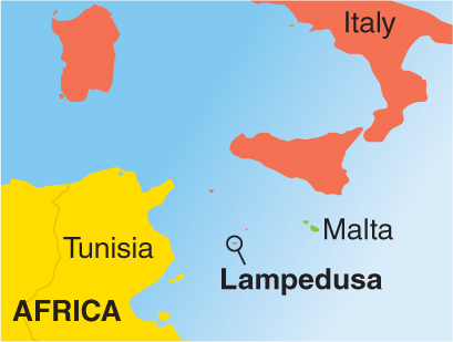
Today, the European Union has expanded to include many of the countries in Eastern Europe, and in principle there is free migration within the European Union. In practice, it can still be difficult for countries to absorb all the workers who want to enter, whether they come from inside or outside the Union. A recent example from Europe is the inflow of migrants from Northern Africa, especially from Tunisia and Libya. During 2011 and 2012, some 58,000 migrants escaped unrest in Africa and sailed on small boats to the island of Lampedusa in Italy. That inflow of migrants has created a situation not unlike the “Mariel boat lift” situation several decades ago in the United States, as discussed at the beginning of the chapter. The inflow has strained the ability of the European Union to maintain passport-free migration between countries. As described in Headlines: Call for Return of Border Controls in Europe, these migrants were not welcome to move freely from Italy to France, where some of them had families or friends.

In the United States, there is a widespread perception among policy makers that the current immigration system is not working and needs to be fixed. A new immigration bill was debated in the U.S. Congress in 2013. As described in Headlines: The Economic Windfall of Immigration Reform, there are several issues that this bill needs to address, related to both illegal and legal immigration.
It is estimated that there are about 12 million illegal immigrants in the United States, many of them from Mexico. Gaining control over U.S. borders is one goal of immigration policy, but focusing on that goal alone obscures the fact that the majority of immigrants who enter the United States each year are legal.
130
There are articles that read like this much of the time...
Political pressures to limit immigration in Europe.
Call for Return of Border Controls in Europe
In 2011, Nicolas Sarkozy, the French president at the time, and Silvio Berlusconi, the Italian prime minister at the time, called for limits on passport-free travel among European Union countries in response to the flood of North African immigrants entering Italy through the island of Lampedusa.
Nicolas Sarkozy and Silvio Berlusconi are expected to call on Tuesday for a partial reintroduction of national border controls across Europe, a move that would put the brakes on European integration and curb passport-free travel for more than 400 million people in 25 countries.
The French president and the Italian prime minister are meeting in Rome after weeks of tension between their two countries over how to cope with an influx of more than 25,000 immigrants fleeing revolutions in north Africa. The migrants, mostly Tunisian, reached the EU by way of Italian islands such as Lampedusa, but many hoped to get work in France where they have relatives and friends.
Earlier this month, Berlusconi’s government outraged several EU governments, including France, by offering the migrants temporary residence permits which, in principle, allowed them to travel to other member states under the Schengen agreement. An Italian junior minister said on Sunday that Rome had so far issued some 8,000 permits and expected the number would rise to 11,000.
Launched in 1995, Schengen allows passport-free travel in most of the EU, Switzerland, Norway and Iceland. But the documents issued by the Italian authorities are only valid if the holders can show they have the means to support themselves, and French police have rounded up or turned back an unknown number of migrants in recent days.
On 17 April, Paris blocked trains crossing the frontier at Ventimiglia in protest at the Italian initiative. “Rarely have the two countries seemed so far apart,” said Le Monde in an editorial on Monday.
Yet, with both leaders under pressure from the far right, French and Italian officials appear to have agreed a common position on amending Schengen so that national border checks can be reintroduced in “special circumstances”.
Source: Excerpted from John Hooper and Ian Traynor, “Sarkozy and Berlusconi to call for return of border controls in Europe,” The Guardian, April 25 2011, electronic edition. Copyright Guardian News & Media Ltd 2011.
Persons seeking to legally enter the United States sometimes must wait a very long time, because under current U.S. law, migrants from any one foreign country cannot number more than 7% of the total legal immigrants into the United States each year. Giovanni Peri, the author of “The Economic Windfall of Immigration Reform” article, proposes that businesses should be allowed to compete for migrants who have the skills needed for the jobs that the businesses have to offer. Firms could, for example, compete by bidding for temporary work permits in auctions. After obtaining the work permits, the firms could then sell them to other firms.7 In this way, the permits would eventually be bought by the firms that valued them most highly, promoting efficiency in the flow of migrants.
Such an auction scheme could be used for seasonal agricultural workers, for example, some of whom legally enter the United States under the H-2A visa program. An auction could also expand the existing H-1B visa program for engineers, scientists, and other skilled workers needed in high-technology industries. The H-1B program was established during the Clinton administration to attract highly skilled immigrants to the United States, and it continues today. According to this article, the inflow of highly skilled immigrants on H-1B visas can explain 10% to 20% of the yearly productivity growth in the United States, as discussed later in the chapter.
131
Peri’s proposal to allow firms to compete for skilled immigrants
The Economic Windfall of Immigration Reform
Writing during the U.S. debate over immigration reform in 2013, Professor Giovanni Peri discusses three principles that reform should follow. He argues that there are large gains from increasing the supply of highly-skilled immigrants to the United States, by allowing firms to bid for temporary work permits.
After months of acrimony, it now appears that immigration reform, and a comprehensive one at that, is within reach. While most of the debates have been about the immediate consequences of any change in policy, the goal should be to promote economic growth over the next 40 years.
Much of the reform debate has centered around granting legal status to undocumented immigrants, conditional upon payment of fees and back taxes. From an economic point of view, this will likely have only a modest impact, especially in the short run. Yet the problem of undocumented immigrants is likely to come back unless we find better ways to legally accommodate new immigrants. Much larger economic gains are achievable if we reorganize the immigration system to do that, following three fundamental principles.
The first is simplification. The current visa system is the accumulation of many disconnected provisions. Some rules, set in the past—such as the 7% limit on permanent permits to any nationality—are arbitrary and produce delays, bottlenecks and inefficiencies…. A more rational approach would have the government set overall targets and simple rules for temporary and permanent working permits, deciding the balance between permits in “skilled” and “unskilled” jobs. But the government should not micromanage permits, rules and limits in specific occupations. Employers compete to hire immigrants, and they are best suited at selecting the individuals who will be the most productive in the jobs that are needed.
The second important principle is that the number of temporary work visas should respond to the demand for labor. Currently the limited number of these visas is set with no consideration for economic conditions. Their number is rarely revised. In periods of high demand, the economic incentives to bypass the limits and hire undocumented workers are large…. [W]e propose that temporary permits to hire immigrants should be made tradable and sold by the government in auctions to employers. Such a “cap and trade” system would ensure efficiency. The auction price of permits would signal the demand for immigrants and guide the upward and downward adjustment of the permit numbers over years.
The third principle governing immigration reform is that scientists, engineers and innovators are the main drivers of productivity and of economic growth…. I have found in a study published in January that foreign scientists and engineers brought into this country under the H1B visa program have contributed to 10%–20% of the yearly productivity growth in the U.S. during the period 1990–2010. This allowed the GDP per capita to be 4% higher that it would have been without them—that’s an aggregate increase of output of $615 billion as of 2010.
Source: Excerpted from Giovanni Peri, “The Economic Windfall of Immigration Reform,” The Wall Street Journal, February 13th 2013. p. A15. Reprinted with permission of The Wall Street Journal, Copyright © (2013) Dow Jones & Company, Inc. All Rights Reserved Worldwide.
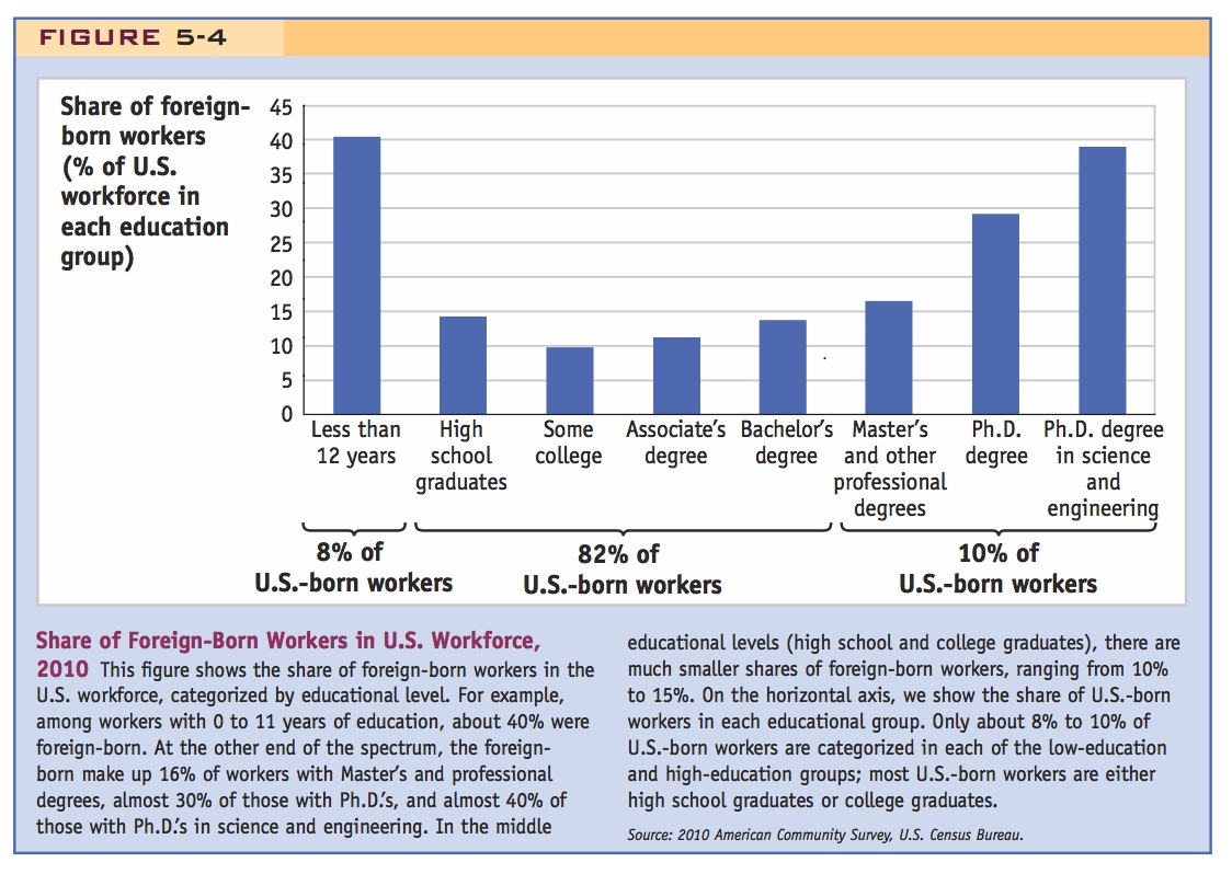
The potential competition that immigrants create for U.S. workers with the same educational level is illustrated in Figure 5-4. On the vertical axis we show the share of immigrants (legal and illegal) as a percentage of the total workforce in the United States with that educational level. For example, from the first bar we see that immigrants account for 40% of the total number of workers in the United States that do not have a high-school education (the remaining 60% are U.S. born). Many of those immigrants without a high-school education are illegal, but we do not know the exact number. We know, however, that the share of high-school dropouts in the U.S.-born workforce is quite small: only 8% of workers born in the United States do not have a high-school education. That percentage is shown on the horizontal axis of Figure 5-4. So, even though illegal immigrants attract much attention in the U.S. debate over immigration, those immigrants with less than high-school education are competing with a small share of U.S.-born workers.
132
As we move to the next bars in Figure 5-4, the story changes. A large portion of U.S.-born workers—82% as shown on the horizontal axis—have completed high school education, may have started college, or graduated with an Associate’s or Bachelor’s degree. The shares of these educational groups that are composed of immigrants are quite small, ranging between 10% and 15% (the remainder being U.S.-born workers). So in these middle levels of education, immigrants are not numerous enough to create a significant amount of competition with U.S.-born workers for jobs.
At the other end of the spectrum, 10% of U.S.-born workers have Master’s degrees or Ph.D.’s. Within this high-education group, foreign-born Master’s-degree holders make up 16% of the U.S. workforce, and foreign-born Ph.D.’s make up nearly 30%, of the U.S. workforce. Furthermore, an even higher fraction of foreign-born immigrants, close to 40%, have Ph.D.’s in science and engineering fields (with slightly more than 60% being U.S. born). To summarize, Figure 5-4 shows that immigrants into the United States compete primarily with workers at the lowest and highest ends of the educational levels and much less with the majority of U.S.-born workers with mid-levels of education.
133
If we extend the specific-factors model to allow for several types of labor distinguished by educational level but continue to treat capital and land as fixed, then the greatest negative impact of immigration on wages would be for the lowest- and highest-educated U.S. workers. That prediction is supported by estimates of the effect of immigration on U.S. wages: from 1990 to 2006, immigration led to a fall in wages of 7.8% for high school dropouts and 4.7% for college graduates. But the impact of immigration on the wages of the majority of U.S. workers (those with mid-levels of education) is much less: wages of high school graduates decreased by 2.2% from 1990 to 2006, and wages of individuals with less than four years of college decreased by less than 1%. The negative impact of immigration on wages is thus fairly modest for most workers and is offset when capital moves between industries, as discussed later in the chapter.
Other Effects of Immigration in the Short Run
3. Other Effects of Immigration in the Short Run
a. Rentals on Capital and Land
The increase in labor raises MPK and MPT so immigration benefits owners of capital and land.
b. Effect of Immigration on Industry Output
Output increases in both sectors. However, this is only true in the short run, not in the long run.
4. Effects of Immigration in the Long Run
Now use HO: Shoes are labor intensive; computers capital intensive
a. Box Diagram
A graphical depiction of the allocation of factors between sectors. Emphasize that different slopes of expansion paths reflect differences in factor intensity.
b. Determination of the Real Wage and Real Rental
Because of diminishing returns, the real rental on capital falls with the capital–labor ratio. Conversely, the real wage falls with the labor–capital ratio. So every point on an expansion path for a sector corresponds to a particular real wage and real rental in that sector.
c. Increase in the Amount of Home Labor
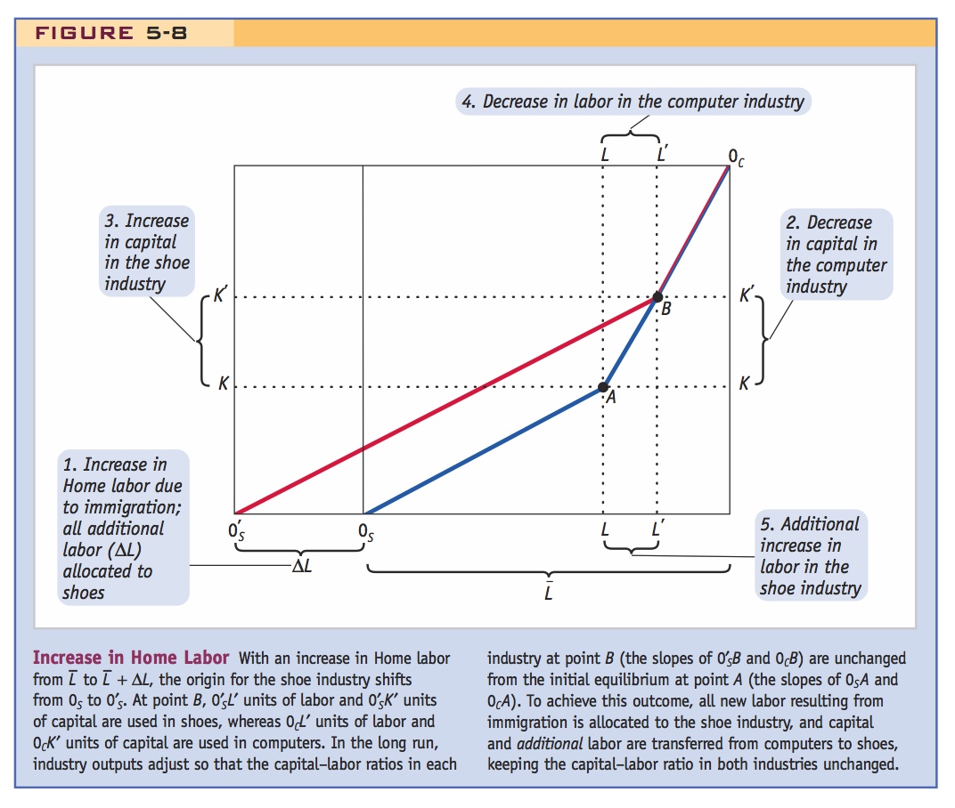
Immigration shifts the box to the right. All of the increase in labor is absorbed in shoes (the labor intensive sector). Since the capital–labor ratios are constant, this requires that capital be shifted away from computers toward shoes. Moreover, since capital–labor ratios have not changed, neither will wages and rentals.
d. Effect of Immigration on Industry Outputs
Immigration causes more capital and labor to be used in the labor-intensive sector. The PPF shifts asymmetrically in favor of the labor intensive good. Therefore, given fixed goods prices, immigration will cause the labor intensive sector to expand, and the capital intensive sector to contract.
5. Rybczynski Theorem:
In the HO model with two goods and two factors, an increase in the amount of a factor will increase the output of the industry using that factor intensively and decrease the output of the other industry.
Because immigration raises output in one sector and reduces it in the other, it will not affect factor returns.
6. Factor Price Insensitivity Theorem:
An increase in the amount of a factor found in an economy can be absorbed by changing the outputs of the industries, without any changes in factor prices.
The United States and Europe have both welcomed foreign workers into specific industries, such as agriculture and the high-tech industry, even though these workers compete with domestic workers in those industries. This observation suggests that there must be benefits to the industries involved. We can measure the potential benefits by the payments to capital and land, which we refer to as “rentals.” We saw in Chapter 3 that there are two ways to compute the rentals: either as the earnings left over in the industry after paying labor or as the marginal product of capital or land times the price of the good produced in each industry. Under either method, the owners of capital and land benefit from the reduction in wages due to immigration.
Rentals on Capital and Land Under the first method for computing the rentals, we take the revenue earned in either manufacturing or agriculture and subtract the payments to labor. If wages fall, then there is more left over as earnings of capital and land, so these rentals are higher. Under the second method for computing rentals, capital and land earn their marginal product in each industry times the price of the industry’s good. As more labor is hired in each industry (because wages are lower), the marginal products of capital and land both increase. The increase in the marginal product occurs because each machine or acre of land has more workers available to it, and that machine or acre of land is therefore more productive. So under the second method, too, the marginal products of capital and land rise and so do their rentals.
Say that this should suggest political fault lines.
From this line of reasoning, we should not be surprised that owners of capital and land often support more open borders, which provide them with foreign workers who can be employed in their industries. The restriction on immigration in a country should therefore be seen as a compromise between entrepreneurs and landowners who might welcome the foreign labor; local unions and workers who view migrants as a potential source of competition leading to lower wages; and the immigrant groups themselves, who if they are large enough (such as the Cuban population in Miami) might also have the ability to influence the political outcome on immigration policy.
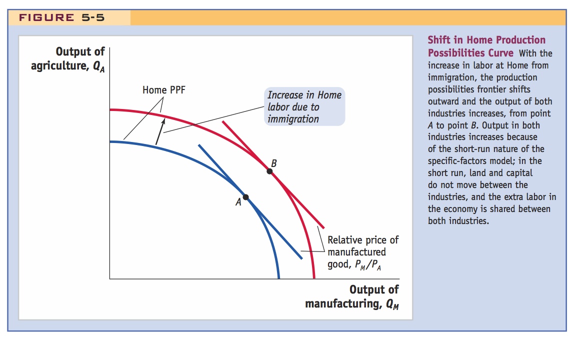
Effect of Immigration on Industry Output One final effect of labor immigration is its effect on the output of the industries. In Figure 5-2, the increase in the labor force due to immigration led to more workers being employed in each of the industries: employment increased from 0ML to 0ML′ in manufacturing and from 0AL to in agriculture. With more workers and the same amount of capital or land, the output of both industries rises. This outcome is shown in Figure 5-5—immigration leads to an outward shift in the production possibilities frontier (PPF). With constant prices of goods (as we assumed earlier, because prices are determined by world supply and demand), the output of the industries rises from point A to point B.
134
Although it may seem obvious that having more labor in an economy will increase the output of both industries, it turns out that this result depends on the short-run nature of the specific-factors model, when capital and land in each industry are fixed. If instead these resources can move between the industries, as would occur in the long run, then the output of one industry will increase but that of the other industry will decline, as we explain in the next section.
Effects of Immigration in the Long Run
We turn now to the long run, in which all factors are free to move between industries. Because it is complicated to analyze a model with three factors of production—capital, land, and labor—all of which are fully mobile between industries, we will ignore land and assume that only labor and capital are used to produce two goods: computers and shoes. The long-run model is just like the Heckscher-Ohlin model studied in the previous chapter except that we now allow labor to move between countries. (Later in the chapter, we allow capital to move between the countries.)
The amount of capital used in computers is KC, and the amount of capital used in shoe production is KS. These quantities add up to the total capital available in the economy: KC + KS =  . Because capital is fully mobile between the two sectors in the long run, it must earn the same rental R in each. The amount of labor used to manufacture computers is LC, and the labor used in shoe production is LS. These amounts add up to the total labor in the economy, LC + LS = , and all labor earns the same wage of W in both sectors.
135

Explain that these L/K ratios are assumed to be constant.
In our analysis, we make the realistic assumption that more labor per machine is used in shoe production than in computer production. That assumption means that shoe production is labor-intensive compared with computer production, so the labor–capital ratio in shoes is higher than it is in computers: LS/KS > LC/KC. Computer production, then, is capital-intensive compared with shoes, and the capital–labor ratio is higher in computers: KC/LC > KS/LS.
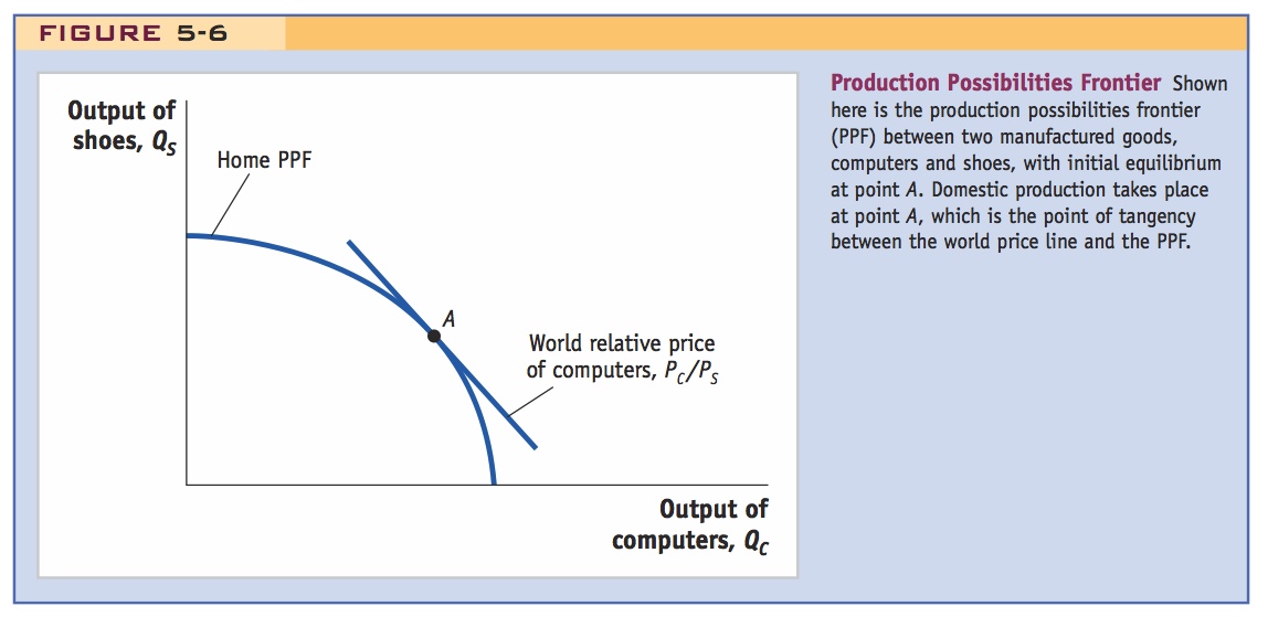
The PPF for an economy producing shoes and computers is shown in Figure 5-6. Given the prices of both goods (determined by supply and demand in world markets), the equilibrium outputs are shown at point A, at the tangency of the PPF and world relative price line. Our goal in this section is to see how the equilibrium is affected by having an inflow of labor into Home as a result of immigration.
Be prepared to go slow on this. Unless students have seen Edgeworth boxes in micro already it will be daunting to some students.
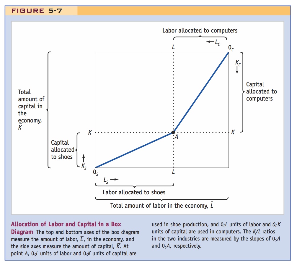
Box Diagram To analyze the effect of immigration, it is useful to develop a new diagram to keep track of the amount of labor and capital used in each industry. Shown as a “box diagram” in Figure 5-7, the length of the top and bottom horizontal axes is the total amount of labor at Home, and the length of the right and left vertical axes is the total amount of capital at Home. A point like point A in the diagram indicates that 0SL units of labor and 0SK units of capital are used in shoes, while 0CL units of labor and 0CK units of capital are used in computers. Another way to express this is that the line 0SA shows the amount of labor and capital used in shoes and the line 0CA shows the amount of labor and capital used in computers.
136
Notice that the line 0SA for shoes is flatter than the line 0CA for computers. We can calculate the slopes of these lines by dividing the vertical distance by the horizontal distance (the rise over the run). The slope of 0SA is 0SK/0SL, the capital–labor ratio used in the shoe industry. Likewise, the slope of 0CA is 0CK/0CL, the capital–labor ratio for computers. The line 0SA is flatter than 0CA, so the capital–labor ratio in the shoe industry is less than that in computers; that is, there are fewer units of capital per worker in the shoe industry. This is precisely the assumption that we made earlier. It is a realistic assumption given that the manufacture of computer components such as semiconductors requires highly precise and expensive equipment, which is operated by a small number of workers. Shoe production, on the other hand, requires more workers and a smaller amount of capital.
If necessary, explain that this follows from constant returns to scale.
Determination of the Real Wage and Real Rental In addition to determining the amount of labor and capital used in each industry in the long run, we also need to determine the wage and rental in the economy. To do so, we use the logic introduced in Chapter 3: the wage and rental are determined by the marginal products of labor and capital, which are in turn determined by the capital–labor ratio in either industry. If there is a higher capital–labor ratio (i.e., if there are more machines per worker), then by the law of diminishing returns, the marginal product of capital and the real rental must be lower. Having more machines per worker means that the marginal product of labor (and hence the real wage) is higher because each worker is more productive. On the other hand, if there is a higher labor–capital ratio (more workers per machine), then the marginal product of labor must be lower because of diminishing returns, and hence the real wage is lower, too. In addition, having more workers per machine means that the marginal product of capital and the real rental are both higher.
137
The important point to remember is that each amount of labor and capital used in Figure 5-7 along line 0SA corresponds to a particular capital–labor ratio for shoe manufacture and therefore a particular real wage and real rental. We now consider how the labor and capital used in each industry will change due to immigration at Home. Although the total amount of labor and capital used in each industry changes, we will show that the capital–labor ratios are unaffected by immigration, which means that the immigrants can be absorbed with no change at all in the real wage and real rental.
Increase in the Amount of Home Labor Suppose that because of immigration, the amount of labor at Home increases from to . This increase expands the labor axes in the box diagram, as shown in Figure 5-8. Rather than allocating labor and capital between the two industries, we must now allocate  labor and capital. The question is how much labor and capital will be used in each industry so that the total amount of both factors is fully employed?
138
You might think that the only way to employ the extra labor is to allocate more of it to both industries (as occurred in the short-run specific-factors model). This outcome would tend to lower the marginal product of labor in both industries and therefore lower the wage. But it turns out that such an outcome will not occur in the long-run model because when capital is also able to move between the industries, industry outputs will adjust to keep the capital–labor ratios in each industry constant. Instead of allocating the extra labor to both industries, all the extra labor (ΔL) will be allocated to shoes, the labor-intensive industry. Moreover, along with that extra labor, some capital is withdrawn from computers and allocated to shoes. To maintain the capital–labor ratio in the computer industry, some labor will also leave the computer industry, along with the capital, and go to the shoe industry. Because all the new workers in the shoe industry (immigrants plus former computer workers) have the same amount of capital to work with as the shoe workers prior to immigration, the capital–labor ratio in the shoe industry stays the same. In this way, the capital–labor ratio in each industry is unchanged and the additional labor in the economy is fully employed.
This outcome is illustrated in Figure 5-8, where the initial equilibrium is at point A. With the inflow of labor due to immigration, the labor axis expands from to + ΔL, from 0S to  . and the origin for the shoe industry shifts from 0S to . Consider point B as a possible new equilibrium. At this point,
  units of labor and
  units of capital are used in shoes, while 0CL′ units of labor and 0CK′ units of capital are used in computers. Notice that the lines 0SA and
  are parallel and have the same slope, and similarly, the lines 0CA and 0CB have the same slope. The extra labor has been employed by expanding the amount of labor and capital used in shoes (the line is longer than 0SA) and contracting the amount of labor and capital used in computers (the line 0CB is smaller than 0CA). That the lines have the same slope means that the capital–labor ratio used in each industry is exactly the same before and after the inflow of labor.
Important result . . .
. . . leading to this one.
What has happened to the wage and rentals in the economy? Because the capital–labor ratios are unchanged in both industries, the marginal products of labor and capital are also unchanged. Therefore, the wage and rental do not change at all because of the immigration of labor! This result is very different from what happens in the short-run specific-factors model, which showed that immigration depressed the wage and raised the rental on capital and land. In the long-run model, when capital can move between industries, an inflow of labor has no impact on the wage and rental. Instead, the extra labor is employed in shoes, by combining it with capital and additional labor that has shifted out of computers. In that way, the capital–labor ratios in both industries are unchanged, as are the wage and rental.
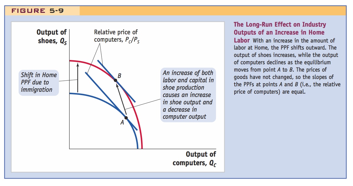
Effect of Immigration on Industry Outputs What is the effect of immigration on the output of each industry? We have already seen from Figure 5-8 that more labor and capital are used in the labor-intensive industry (shoes), whereas less labor and capital are used in the capital-intensive industry (computers). Because the factors of production both increase or both decrease, it follows that the output of shoes expands and the output of computers contracts.
This outcome is shown in Figure 5-9, which shows the outward shift of the PPF due to the increase in the labor endowment at Home. Given the prices of computers and shoes, the initial equilibrium was at point A. At this point, the slope of the PPF equals the relative price of computers, as shown by the slope of the line tangent to the PPF. With unchanged prices for the goods, and more labor in the economy, the equilibrium moves to point B, with greater output of shoes but reduced output of computers. Notice that the slope of the PPFs at points A and B is identical because the relative price of computers is unchanged. As suggested by the diagram, the expansion in the amount of labor leads to an uneven outward shift of the PPF—it shifts out more in the direction of shoes (the labor-intensive industry) than in the direction of computers. This asymmetric shift illustrates that the new labor is employed in shoes and that this additional labor pulls capital and additional labor out of computers in the long run, to establish the new equilibrium at point B. The finding that an increase in labor will expand one industry but contract the other holds only in the long run; in the short run, as we saw in Figure 5-5, both industries will expand. This finding, called the Rybczynski theorem, shows how much the long-run model differs from the short-run model. The long-run result is named after the economist T. N. Rybczynski, who first discovered it.
139
Rybczynski Theorem
The formal statement of the Rybczynski theorem is as follows: in the Heckscher-Ohlin model with two goods and two factors, an increase in the amount of a factor found in an economy will increase the output of the industry using that factor intensively and decrease the output of the other industry.
We have proved the Rybczynski theorem for the case of immigration, in which labor in the economy grows. As we find later in the chapter, the same theorem holds when capital in the economy grows: in this case, the industry using capital intensively expands and the other industry contracts.8
140
Effect of Immigration on Factor Prices The Rybczynski theorem, which applies to the long-run Heckscher-Ohlin model with two goods and two factors of production, states that an increase in labor will expand output in one industry but contract output in the other industry. Notice that the change in outputs in the Rybczynski theorem goes hand in hand with the previous finding that the wage and rental will not change due to an increase in labor (or capital). The reason that factor prices do not need to change is that the economy can absorb the extra amount of a factor by increasing the output of the industry using that factor intensively and reducing the output of the other industry. The finding that factor prices do not change is sometimes called the factor price insensitivity result.
Factor Price Insensitivity Theorem
Students will naturally expect wages to change, so emphasize how powerful and surprising this result is.
The factor price insensitivity theorem states that: in the Heckscher-Ohlin model with two goods and two factors, an increase in the amount of a factor found in an economy can be absorbed by changing the outputs of the industries, without any change in the factor prices.
The applications that follow offer evidence of changes in output that absorb new additions to the labor force, as predicted by the Rybczynski theorem, without requiring large changes in factor prices, as predicted by the factor price insensitivity result.
Expansion of unskilled labor-intensive industries and contraction of skilled labor-intensive industries in Miami after Mariel may support Rybczynski.
The Effects of the Mariel Boat Lift on Industry Output in Miami
Now that we have a better understanding of long-run adjustments due to changes in factor endowments, let us return to the case of the Mariel boat lift to Miami in 1980. We know that the Cuban refugees were less skilled than the average labor force in Miami. According to the Rybczynski theorem, then, we expect some unskilled-labor–intensive industry, such as footwear or apparel, to expand. In addition, we expect that some skill-intensive industry, such as the high-tech industry, will contract. Figure 5-10 shows how this prediction lines up with the evidence from Miami and some comparison cities.9
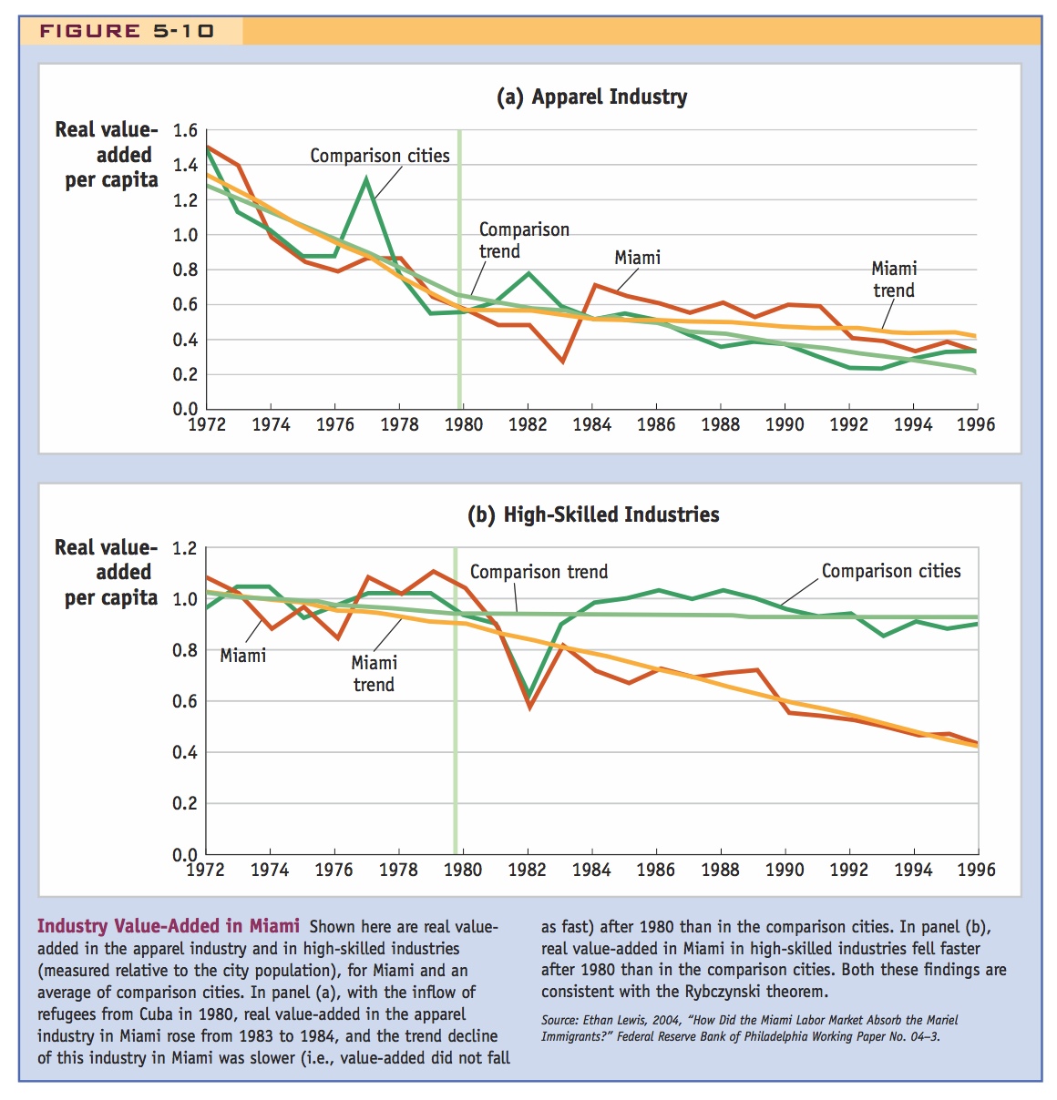
Panel (a) of Figure 5-10 shows real value-added in the apparel industry for Miami and for an average of comparison cities. Real value-added measures the payments to labor and capital in an industry corrected for inflation. Thus, real value-added is a way to measure the output of the industry. We divide output by the population of the city to obtain real value-added per capita, which measures the output of the industry adjusted for the city size.
Panel (a) shows that the apparel industry was declining in Miami and the comparison cities before 1980. After the boat lift, the industry continued to decline but at a slower rate in Miami; the trend of output per capita for Miami has a smaller slope (and hence a smaller rate of decline in output) than that of the trend for comparison cities from 1980 onward. Notice that there is an increase in industry output in Miami from 1983 to 1984 (which may be due to new data collected that year), but even when averaging this out as the trend lines do, the industry decline in Miami is slightly slower than in the comparison cities after 1980. This graph provides some evidence of the Rybczynski theorem at work: the reduction in the apparel industry in Miami was slower than it would have been without the inflow of immigrants.
141
What about the second prediction of the Rybczynski theorem: Did the output of any other industry in Miami fall because of the immigration? Panel (b) of Figure 5-10 shows that the output of a group of skill-intensive industries (including motor vehicles, electronic equipment, and aircraft) fell more rapidly in Miami after 1980. These data may also provide some evidence in favor of the Rybczynski theorem. However, it also happened that with the influx of refugees, there was a flight of homeowners away from Miami, and some of these were probably high-skilled workers. So the decline in the group of skill-intensive industries, shown in panel (b), could instead be due to this population decline. The change in industry outputs in Miami provides some evidence in favor of the Rybczynski theorem. Do these changes in industry outputs in Miami also provide an adequate explanation for why wages of unskilled workers did not decline, or is there some other explanation? An alternative explanation for the finding that wages did not change comes from comparing the use of computers in Miami with national trends. Beginning in the early 1980s, computers became increasingly used in the workplace. The adoption of computers is called a “skill-biased technological change.” That is, computers led to an increase in the demand for high-skilled workers and reduced the hiring of low-skilled workers. This trend occurred across the United States and in other countries.
142
In Miami, however, computers were adopted somewhat more slowly than in cities with similar industry mix and ethnic populations. One explanation for this finding is that firms in many industries, not just apparel, employed the Mariel refugees and other low-skilled workers rather than switching to computer technologies. Evidence to support this finding is that the Mariel refugees were, in fact, employed in many industries. Only about 20% worked in manufacturing (5% in apparel), and the remainder worked in service industries. The idea that the firms may have slowed the adoption of new technologies to employ the Mariel emigrants is hard to prove conclusively, however. We suggest it here as an alternative to the Rybczynski theorem to explain how the refugees could be absorbed across many industries rather than just in the industries using unskilled labor, such as apparel.
HO's prediction holds on average, wages of skilled labor may change relative to unskilled. Conclusion might remind students of some explanations for the Leontief paradox.
Controlling to keep the capital–labor ratio constant, wages in the United States were roughly constant after immigration. However, wages fell for the least and the most educated workers. This could be explained by allowing for imperfect substitutability between the U.S. and immigrant worker.
Immigration and U.S. Wages, 1990–2006
In 1980, the year of the Mariel boat lift, the percentage of foreign-born people in the U.S. population was 6.2%. The percentage grew to 9.1% in 1990 and then to 13.0% in 2005, so there was slightly more than a doubling of foreign-born people in 25 years.10 That period saw the greatest recent increase in foreign-born people in the United States, and by 2010 the percentage had grown only slightly more, to 13.5%. How did the wave of immigration prior to 2006 affect U.S. wages?
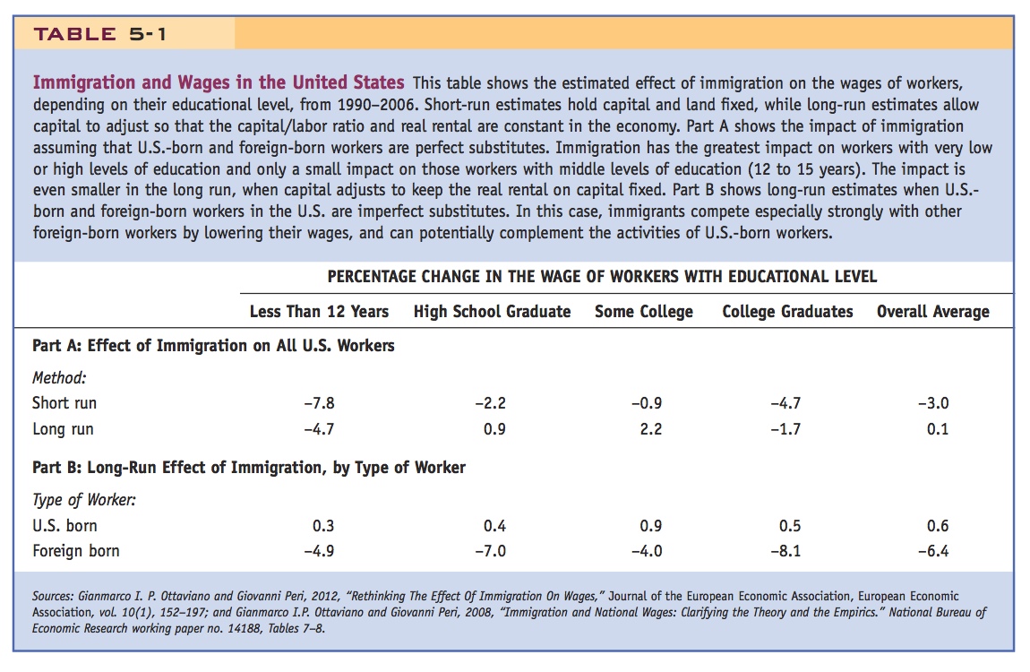
Part A of Table 5-1 reports the estimated impact of the immigration from 1990 to 2006 on the wages of various workers, distinguished by their educational level. The first row in part A summarizes the estimates from the specific-factors model, when capital and land are kept fixed within all industries. As we discussed in an earlier application, the greatest negative impact of immigration is on native-born workers with less than 12 years of education, followed by college graduates, and then followed by high school graduates and those with some college. Overall, the average impact of immigration on U.S. wages over the period of 1990–2006 was −3.0%. That is, wages fell by 3.0%, consistent with the specific-factors model.
143
A different story emerges, however, if instead of keeping capital fixed, we hold constant the capital–labor ratio in the economy and the real rental on capital. Under this approach, we allow capital to grow to accommodate the inflow of immigrants, so that there is no change in the real rental. This approach is similar to the long-run model we have discussed, except that we now distinguish several types of labor by their education levels. In the second row of part A, we see that total U.S. immigration had a negative impact on workers with the lowest and highest levels of education and a positive impact on the other workers (due to the growth in capital). With these new assumptions, we see that the average U.S. wage rose by 0.1% because of immigration (combined with capital growth), rather than falling by 3.0%.
The finding that the average U.S. wage is nearly constant in the long run (rising by just 0.1%) is similar to our long-run model in which wages do not change because of immigration. However, the finding that some workers gain (wages rise for the middle education levels) and others lose (wages fall for the lowest and the highest education levels) is different from our long-run model. There are two reasons for this outcome. First, as we already noted, Table 5-1 categorizes workers by different education levels. Even when the overall capital–labor ratio is fixed, and the real rental on capital is fixed, it is still possible for the wages of workers with certain education levels to change. Second, we can refer back to the U-shaped pattern of immigration shown in Figure 5-4, where the fraction of immigrants in the U.S. workforce is largest for the lowest and highest education levels. It is not surprising, then, that these two groups face the greatest loss in wages due to an inflow of immigrants.
144
We can dig a little deeper to better understand the long-run wage changes in part A. In part A, we assumed that U.S.-born workers and foreign-born workers in each education level are perfect substitutes, that is, they do the same types of jobs and have the same abilities. In reality, evidence shows that U.S. workers and immigrants often end up doing different types of jobs, even when they have similar education. In part B of Table 5-1, we build in this realistic feature by treating U.S.-born workers and foreign-born workers in each education level as imperfect substitutes. Just as the prices of goods that are imperfect substitutes (for example, different types of cell phones) can differ, the wages of U.S.-born and foreign-born workers with the same education can also differ. This modification to our assumptions leads to a substantial change in the results.
In part B of Table 5-1, we find that immigration now raises the wages of all U.S.-born workers in the long run, by 0.6% on average. That slight rise occurs because the U.S-born and foreign-born workers are doing different jobs that can complement one another. For example, on a construction site, an immigrant worker with limited language skills can focus on physical tasks, while a U.S. worker can focus on tasks involving personal interaction. Part B shows another interesting outcome: the 1990–2006 immigration had the greatest impact on the wages of all other foreign-born workers, whose wages fell by an average of 6.4% in the long run. When we allow for imperfect substitution between U.S.-born and foreign-born workers, immigrants compete especially strongly with other foreign-born workers, and can potentially complement the activities of U.S.-born workers. Contrary to popular belief, immigrants don’t necessarily lower the wages for U.S. workers with similar educational backgrounds. Instead, immigrants can raise wages for U.S. workers if the two groups are doing jobs that are complementary.
Emphasize that this has important policy implications.