1 A Model of Offshoring
1. Rank production activities, first by order in production, then in terms of the relative amounts of high-skilled and low-skilled labor it requires.
2. Value Chain of Activities
Each activity contributes to the value of the combined product. Some can be sent overseas. Ranking them by relative skill level will help predict which will be done abroad.
a. Relative Wage of Skilled Workers
Wages are lower abroad than at home, for both low-skill and high-skill workers However, the relative wage of low-skill workers is lower abroad.
b. Costs of Capital and Trade
A company can benefit from lower wage costs by offshoring. However, offshoring also incurs higher capital and trade costs than domestic production. For simplicity, assume that these trade costs apply uniformly across the value chain.
c. Slicing the Value Chain
Which activities will the firm send offshore? The ones that are least-skilled and most labor-intensive—“slicing the value chain.”
d. Relative Demand for Skilled Labor
Relative demand for skilled labor in each country is negatively sloped because a higher relative wage for skilled labor would induce substitution towards less skilled labor. Assume positively sloped relative supply curves for skilled labor.
3. Changing the Costs of Trade
Suppose that trade costs fall (e.g., NAFTA or Indian deregulation):
a. Change in Home Labor Demand and Relative Wage. Offshoring from Home increases because more less-skilled work is sent abroad. This raises the relative demand for skilled labor at Home, increasing the relative wage of skilled workers.
b. Change in Foreign Labor Demand and Relative Wage. Conversely, the new jobs offshored to Foreign are more skilled than the jobs that were initially offshored. So the relative demand for skilled labor abroad also increases, raising the relative wage of skilled workers abroad too. Notice that the relative demand for skilled labor increases in both countries. This could not occur in HO.
To develop a model of offshoring, we need to identify all the activities involved in producing and marketing a good or service. These activities are illustrated in Figure 7-1. Panel (a) describes the activities in the order in which they are performed (starting with research and development [R&D] and ending with marketing and after-sales service). For instance, in producing a television, the design and engineering are developed first; components such as wiring, casing, and screens are manufactured next; and finally the television is assembled into its final version and sold to consumers.

For the purpose of building a model of offshoring, however, it is more useful to line up the activities according to the ratio of high-skilled/low-skilled labor used, as in panel (b). We start with the less skilled activities, such as the manufacture and assembly of simple components (like the case or the electric cord for the television), then move to more complex components (like the screen). Next are the supporting service activities such as accounting, order processing, and product service (sometimes called “back-office” activities because the customer does not see them). Finally, we come to activities that use more skilled labor, such as marketing and sales (“front-office” activities), and those that use the most skilled labor such as R&D.
Value Chain of Activities
The whole set of activities that we have illustrated in Figure 7-1 is sometimes called the value chain for the product, with each activity adding more value to the combined product. All these activities do not need to be done in one country—a firm can transfer some of these activities abroad by offshoring them when it is more economical to do so. By lining up the activities in terms of the relative amount of skilled labor they require, we can predict which activities are likely to be transferred abroad. This prediction depends on several assumptions, which follow.
201
Relative Wage of Skilled Workers Let WL be the wage of low-skilled labor in Home and WH the wage of high-skilled labor. Similarly, let W*L and W*H be the wages of low-skilled and high-skilled workers in Foreign. Our first assumption is that Foreign wages are less than those at Home, W*L < WL and W*H < WH, and that the relative wage of low-skilled labor is lower in Foreign than at Home, so W*L/W*H < WL/WH. This assumption is realistic because low-skilled labor in developing countries receives especially low wages.
Costs of Capital and Trade As the firm considers sending some activities abroad, it knows that it will lower its labor costs because wages in Foreign are lower. However, the firm must also take into account the extra costs of doing business in Foreign. In many cases, the firm pays more to capital through (1) higher prices to build a factory or higher prices for utilities such as electricity and fuel; (2) extra costs involved in transportation and communication, which will be especially high if Foreign is still developing roads, ports, and telephone capabilities; and (3) the extra costs from tariffs if Foreign imposes taxes on goods (such as component parts) when they come into the country. We lump together costs 2 and 3 into what we call “trade costs.”
Higher capital and trade costs in Foreign can prevent a Home firm from offshoring all its activities abroad. In making the decision of what to offshore, the Home firm will balance the savings from lower wages against the extra costs of capital and trade.
Our second assumption is that these extra costs apply uniformly across all the activities in the value chain; that is, these extra costs add, say, 10% to each and every component of operation in Foreign as compared with Home. Unlike our assumption about relative wages in Home and Foreign, this assumption is a bit unrealistic. For instance, the extra costs of transportation versus those of communication are quite different in countries such as China and India; good roads for transport have developed slowly, while communications technology has developed rapidly. As a result, technology in telephones is advanced in those countries, so cell phones are often cheaper there than in the United States and Europe. In this case, the higher infrastructure costs will affect the activities that rely on transportation more than activities that rely on communication.
Slicing the Value Chain Now suppose that the Home firm with the value chain in Figure 7-1, panel (b), considers transferring some of these activities from Home to Foreign. Which activities will be transferred? Based on our assumptions that W*L/W*H < WL/WH and that the extra costs of capital and trade apply uniformly, it makes sense for the firm to send abroad the activities that are the least skilled and labor-intensive and keep at Home the activities that are the most skilled and labor-intensive. Looking at Figure 7-1, all activities to the left of the vertical line A might be done in Foreign, for example, whereas those activities to the right of the vertical line will be done in Home. We can refer to this transfer of activities as “slicing the value chain.”4
202
Students may ask how exactly A is determined? The answer requires specifying the cost function and thinking along the lines of H-O with a continuum of goods. So just wave your hands, since the result makes sense intuitively.
By now they should be familiar with relative demand and supply curves, but make sure they understand the intuition for the slopes.
Activities to the left of line A are sent abroad because the cost savings from paying lower wages in Foreign are greatest for activities that require less skilled labor. Because the extra costs of capital and trade are uniform across activities, the cost savings on wages are most important in determining which activities to transfer and which to keep at Home.
Relative Demand for Skilled Labor Now that we know the division of activities between Home and Foreign, we can graph the demand for labor in each country, as illustrated in Figure 7-2. For Home, we add up the demand for high-skilled labor H and low-skilled labor L for all the activities to the right of line A in Figure 7-1, panel (b). Taking the ratio of these, in panel (a) we graph the relative demand for skilled labor at Home H/L against the relative wage WH/WL. This relative demand curve slopes downward because a higher relative wage for skilled labor would cause Home firms to substitute less skilled labor in some activities. For example, if the relative wage of skilled labor increased, Home firms might hire high school rather than college graduates to serve on a sales force and then train them on the job.

In Foreign, we add up the demand for high-skilled labor H* and for low-skilled labor L* for all the activities to the left of line A*. Panel (b) graphs the relative demand for skilled labor in Foreign H*/L* against the relative wage W*H/W*L. Again, this curve slopes downward because a higher relative wage for skilled labor would cause Foreign firms to substitute less skilled labor in some activities. In each country, we can add a relative supply curve to the diagram, which is upward-sloping because a higher relative wage for skilled labor causes more skilled individuals to enter this industry. For instance, if the high-skilled wage increases relative to the low-skilled wage in either country, then individuals will invest more in schooling to equip themselves with the skills necessary to earn the higher relative wage.
203
The intersection of the relative demand and relative supply curves, at points A and A*, gives the equilibrium relative wage in this industry in each country and the equilibrium relative employment of high-skilled/low-skilled workers. Starting at these points, next we study how the equilibrium changes as Home offshores more activities to Foreign.
Changing the Costs of Trade
Suppose now that the costs of capital or trade in Foreign fall. For example, the North American Free Trade Agreement (NAFTA) lowered tariffs charged on goods crossing the U.S.–Mexico border. This fall in trade costs made it easier for U.S. firms to offshore to Mexico. And even before NAFTA, Mexico had liberalized the rules concerning foreign ownership of capital there, thereby lowering the cost of capital for U.S. firms. Another example is India, which in 1991 eliminated many regulations that had been hindering businesses, communications, and foreign investment. Before 1991 it was difficult for a new business to start, or even to secure a phone or fax line in India; after 1991 the regulations on domestic and foreign-owned business were simplified, and communication technology improved dramatically with cell phones and fiber-optic cables. These policy changes made India more attractive to foreign investors and firms interested in offshoring.
Change in Home Labor Demand and Relative Wage When the costs of capital or trade decline in Foreign, it becomes desirable to shift more activities in the value chain from Home to Foreign. Figure 7-3 illustrates this change with the shift of the dividing line from A to B. The activities between A and B, which used to be done at Home, are now done in Foreign. As an example, consider the transfer of television production from the United States to Mexico. As U.S. firms first shifted manufacturing to Mexico, the chassis of the televisions were constructed there. Later on, electronic circuits were constructed in Mexico, and later still the picture tubes were manufactured there.5

204
How does this increase in offshoring affect the relative demand for skilled labor in each country? First consider the Home country. Notice that the activities no longer performed at Home (i.e., those between A and B) are less skill-intensive than the activities still done there (those to the right of B). This means that the activities now done at Home are more skilled and labor-intensive, on average, than the activities formerly done at Home. For this reason, the relative demand for skilled labor at Home will increase, and the Home demand curve will shift to the right, as shown in Figure 7-4, panel (a). Note that this diagram does not show the absolute quantity of labor demanded, which we expect would fall for both high-skilled and low-skilled labor when there is more offshoring; instead, we are graphing the relative demand for high-skilled/low-skilled labor, which increases because the activities still done at Home are more skill-intensive than before the decrease in trade and capital costs. With the increase in the relative demand for skilled labor, the equilibrium will shift from point A to point B at Home; that is, the relative wage of skilled labor will increase because of offshoring.

Change in Foreign Labor Demand and Relative Wage Now let’s look at what happens in Foreign when Home offshores more of its production activities to Foreign. How will offshoring affect the relative demand for labor and relative wage in Foreign? As we saw in Figure 7-3, the activities that are newly offshored to Foreign (those between A and B) are more skill-intensive than the activities that were initially offshored to Foreign (those to the left of A). This means that the range of activities now done in Foreign is more skilled and labor-intensive, on average, than the set of activities formerly done there. For this reason, the relative demand for skilled labor in Foreign also increases, and the Foreign demand curve shifts to the right, as shown in panel (b) of Figure 7-4. With this increase in the relative demand for skilled labor, the equilibrium shifts from point A* to point B*. As a result of Home’s increased offshoring to Foreign, then, the relative wage of skilled labor increases in Foreign. The conclusion from our model is that both countries experience an increase in the relative wage of skilled labor because of increased offshoring.
205
That relative demand for skilled labor increases at Home is fairly obvious, but that it will abroad too is more surprising. It also leads to strong empirical hypotheses. Be sure to employ the reasoning in the next paragraph to develop the intuition.
It might seem surprising that a shift of activities from one country to the other can increase the relative demand for skilled labor in both countries. An example drawn from your classroom experience might help you to understand how this can happen. Suppose you have a friend who is majoring in physics but is finding it difficult: she is scoring below average in a physics class that she is taking. So you invite her to join you in an economics class, and it turns out that your friend has a knack for economics: she scores above average in that class. How does your friend’s transfer from physics to economics affect the class averages? Because she was performing below average in the physics class, when she leaves the class, her departure raises the class average (computed now using the students still there, not including her). Because your friend performs better than average in the economics class, her arrival raises the class average there, too (computed using everyone, including your friend). Thus, your friend’s move from one class to another raises the average in both classes.
This result is just like the logic of the offshoring model: as activities in the middle of the value chain are shifted from Home to Foreign, they raise the relative demand for skilled labor in both countries because these activities are the least skill-intensive of those formerly done at Home but the most skill-intensive of tasks done in Foreign. That is why the relative demand for skilled labor increases in both countries, along with the relative wage of skilled labor. This result is one of the most important predictions from our offshoring model and it would not occur in our earlier models of trade, such as the Heckscher-Ohlin model.6 We now turn to evidence from the United States and Mexico to see whether this prediction is borne out.
Relative wages of skilled workers have increased in the U.S. and in Mexico. It could be because of offshoring, or because of skill-based technological change.
Change in Relative Wages Across Countries
Since the early 1980s, the wages of high-skilled workers have risen relative to those of low-skilled workers in many countries. The relative wage of skilled workers in industrial countries (such as the United States, Australia, Canada, Japan, Sweden, and the United Kingdom) and in developing countries (such as Hong Kong, Chile, and Mexico) has increased. Our offshoring model predicts that the relative wage of skilled workers will rise in both the country doing the offshoring and the country receiving the new activities. At first glance, that prediction seems to be consistent with the change in wages that has actually occurred. Let us dig more deeply, however, using evidence from the United States and Mexico, to see what the change in wages has been and whether it is due to offshoring.
206
Change in Relative Wages in the United States
To measure the wages of skilled and low-skilled workers, we can use data from the manufacturing sector on “production” and “nonproduction” workers. As their name suggests, production workers are involved in the manufacture and assembly of goods, whereas nonproduction workers are involved in supporting service activities. Firms are required to report wages for both types of workers. We could also call these two types of workers “blue collar” and “white collar.” Generally, nonproduction workers require more education, and so we will treat these workers as “high-skilled,” whereas the production workers are treated here as “low-skilled” workers.7
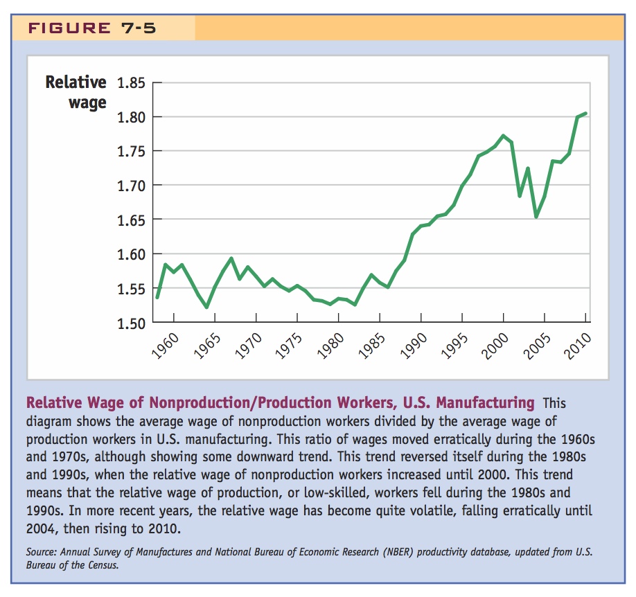
Relative Wage of Nonproduction Workers Figure 7-5 shows the average annual earnings of nonproduction workers relative to production workers (analogous to the ratio of high-skilled to low-skilled wages, or WH/WL) in U.S. manufacturing from 1958 to 2010. We see that relative earnings moved erratically from 1958 to 1967, and that from 1968 to about 1982, relative wages were on a downward trend. It is generally accepted that the relative wage fell during this period because of an increase in the supply of college graduates, skilled workers who moved into nonproduction jobs (the increase in supply would bring down the nonproduction wage, so the relative wage would also fall). Starting in 1982, however, this trend reversed itself and the relative wage of nonproduction workers increased steadily to 2000. Since that time the relative wage fell erratically until 2004, and then rose again to 2010.
207
Relative Employment of Nonproduction Workers In Figure 7-6, we see that there was a steady increase in the ratio of nonproduction to production workers employed in U.S. manufacturing until about 1992. Such a trend indicates that firms were hiring fewer production, or low-skilled workers, relative to nonproduction workers. During the 1990s the ratio of nonproduction to production workers fell until 1998, after which relative employment rose again.

Summary: The fact we want to explain is that both the relative wage and employment of skilled workers increased. This can ONLY be explained by an increase in relative demand. But what caused it?
The increase in the relative supply of college graduates from 1968 to 1982 is consistent with the reduction in the relative wage of nonproduction workers, as shown in Figure 7-5, and with the increase in their relative employment, as shown in Figure 7-6. After 1982, however, the story changes. We would normally think that the rising relative wage of nonproduction workers should have led to a shift in employment away from nonproduction workers, but it did not; as shown in Figure 7-6, the relative employment of nonproduction workers continued to rise from 1980 to about 1992, then fell until 1998. How can there be both an increase in the relative wage and an increase in the relative employment of nonproduction workers? The only explanation consistent with these facts is that during the 1980s there was an outward shift in the relative demand for nonproduction (skilled) workers, which led to a simultaneous increase in their relative employment and in their wages.
208
This conclusion is illustrated in Figure 7-7, in which we plot the relative wage of nonproduction workers and their relative employment from 1979 to 1990. As we have already noted, both the relative wage and relative employment of nonproduction workers rose during the 1980s. The only way this pattern can be consistent with a supply and demand diagram is if the relative demand curve for skilled labor increases, as illustrated. This increased demand would lead to an increase in the relative wage for skilled labor and an increase in its relative employment, the pattern seen in the data for the United States.

Two explanations: (1) Offshoring, (2) Skill-biased technological
Explanations What factors can lead to an increase in the relative demand for skilled labor? One explanation is offshoring. An increase in demand for high-skilled workers, at the expense of low-skilled workers, can arise from offshoring, as shown by the rightward shift in the relative demand for skilled labor in Figure 7-4, panel (a). The evidence from the manufacturing sector in the United States is strongly consistent with our model of offshoring.
There is, however, a second possible explanation for the increase in the relative demand for skilled workers in the United States. In the 1980s personal computers began to appear in the workplace. The addition of computers in the workplace can increase the demand for skilled workers to operate them. The shift in relative demand toward skilled workers because of the use of computers and other high-tech equipment is called skill-biased technological change. Given these two potential explanations for the same observation, how can we determine which of these factors was most responsible for the actual change in wages?
209
Answering this question has been the topic of many research studies in economics. The approach that most authors take is to measure skill-biased technological change and offshoring in terms of some underlying variables. For skill-biased technological change, for example, we might use the amount of computers and other high-technology equipment used in manufacturing industries. For offshoring, we could use the imports of intermediate inputs into manufacturing industries. By studying how the use of high-tech equipment and the imports of intermediate inputs have grown and comparing this with the wage movements in industries, we can determine the contribution of each factor toward explaining the wage movements.
The results from one study of this type are shown in Table 7-1. The goal of this study was to explain two observations. First, it sought to explain the increase in the share of total wage payments going to nonproduction (high-skilled) labor in U.S. manufacturing industries from 1979 to 1990 (part A). Because wage payments equal the wage times the number of workers hired, this statistic captures both the rising relative wage and the rising relative employment of skilled workers. Second, the study analyzed the increase in the relative wage of nonproduction labor in particular over the same period (part B).8
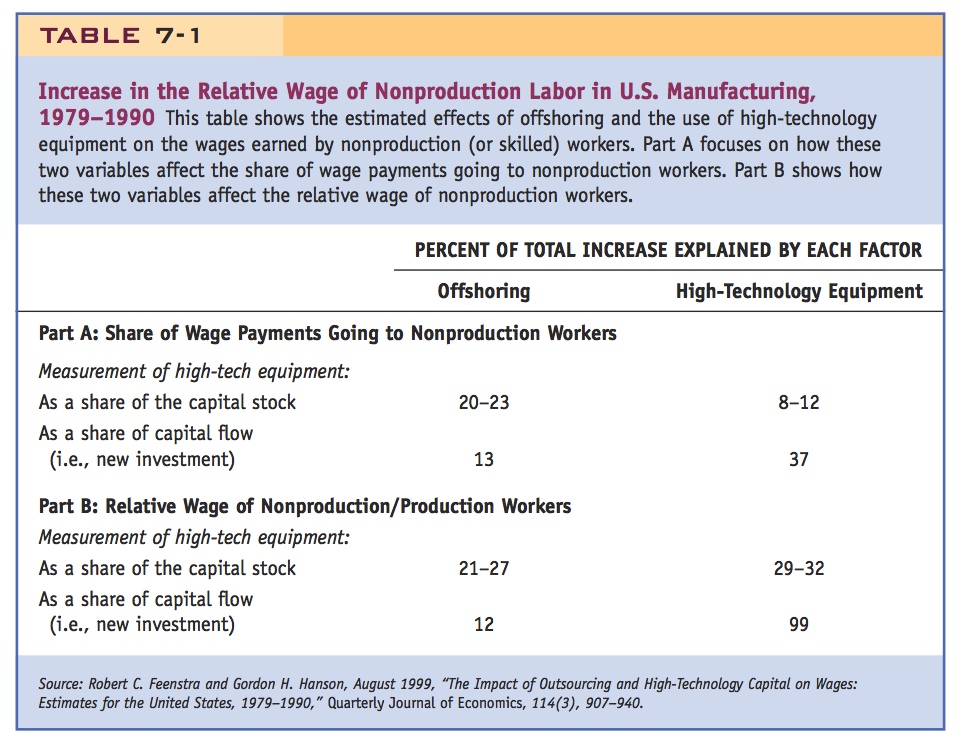
The study considered two possible explanations for the two observations: offshoring and the use of high-tech equipment such as computers. Offshoring was measured as the intermediate inputs imported by each industry. For example, the U.S. auto industry builds seats, dashboards, and other car parts in Mexico and then imports these for assembly in the United States. In addition, high-technology equipment can be measured in two ways: either as a fraction of the total capital equipment installed in each industry or as a fraction of new investment in capital that is devoted to computers and other high-tech devices. In the first method, high-tech equipment is measured as a fraction of the capital stock, and in the second method, high-tech equipment is measured as a fraction of the annual flow of new investment. In the early 1980s a large portion of the flow of new investment in some industries was devoted to computers and other high-tech devices, but a much smaller fraction of the capital stock consisted of that equipment. In Table 7-1, we report results from both measures because the results differ depending on which measure is used.
Using the first measure of high-tech equipment (as a fraction of the capital stock), the results in the first row of part A show that between 20% and 23% of the increase in the share of wage payments going to the nonproduction workers can be explained by offshoring, and between 8% and 12% of that increase can be explained by the growing use of high-tech capital. The remainder is unexplained by these two factors. Thus, using the first measure of high-tech equipment, it appears that offshoring was more important than high-tech capital in explaining the change in relative demand for skilled workers.
210
The story is different, however, if we instead use offshoring and the second measure of high-tech equipment (a fraction of new investment), as shown in the second row of part A. In that case, offshoring explains only 13% of the increase in the nonproduction share of wages, whereas high-tech investment explains 37% of that increase. So we see from these results that both offshoring and high-tech equipment are important explanations for the increase in the relative wage of skilled labor in the United States, but which one is most important depends on how we measure the high-tech equipment.
In part B, we repeat the results but now try to explain the increase in the relative wage of nonproduction workers. Using the first measure of high-tech equipment (a fraction of the capital stock), the results in the first row of part B show that between 21% and 27% of the increase in the relative wage of nonproduction workers can be explained by offshoring, and between 29% and 32% of that increase can be explained by the growing use of high-tech capital. In the second row of part B, we use the other measure of high-tech equipment (a fraction of new investment). In that case, the large spending on high-tech equipment in new investment can explain nearly all (99%) of the increased relative wage for nonproduction workers, leaving little room for offshoring to play much of a role (it explains only 12% of the increase in the relative wage). These results are lopsided enough that we might be skeptical of using new investment to measure high-tech equipment and therefore prefer the results in the first rows of parts A and B, using the capital stocks.
So there is no consensus about which is the culprit.
Summing up, we conclude that both offshoring and high-tech equipment explain the increase in the relative wage of nonproduction/production labor in U.S. manufacturing, but it is difficult to judge which is more important because the results depend on how we measure the high-tech equipment.
211
Change in Relative Wages in Mexico
Our model of offshoring predicts that the relative wage of skilled labor will rise in both countries. We have already seen (in Figure 7-5) that the relative wage of nonproduction (skilled) labor rises in the United States. But what about for Mexico?
In Figure 7-8, we show the relative wage of nonproduction/production labor in Mexico from 1964 to 2000. The data used in Figure 7-8 come from the census of industries in Mexico, which occurred infrequently, so there are only a few turning points in the graph in the early years. We can see that the relative wage of nonproduction workers fell from 1964 to 1984, then rose until 1996, leveling out thereafter. The fall in the relative wage from 1964 to 1984 is similar to the pattern in the United States and probably occurred because of an increased supply of skilled labor in the workforce. More important, the rise in the relative wage of nonproduction workers from 1984 to 1996 is also similar to what happened in the United States and illustrates the prediction of our model of offshoring: that relative wages move in the same direction in both countries.

As the model predicts!
Maybe this leveling off had something to do with the peso crisis, so the increase in the relative wage would have continued without it.
The leveling off of the relative wage of nonproduction workers in Mexico occurred in 1996, two years after the North American Free Trade Agreement (NAFTA) established free trade between the United States, Canada, and Mexico. The tariff reductions on imports from Mexico to the United States began in 1994 and were phased in over the next ten years. Tariffs on imports from the United States and other countries into Mexico had been reduced much earlier, however—right around the 1984 turning point that we see in Figure 7-8. According to one study:9
212
In 1985, in the midst of the debt crisis and as a result of the collapse of the oil price, Mexico initiated an important process of trade liberalization. In that year, Mexico implemented a considerable unilateral reduction in trade barriers and announced its intention to participate in the General Agreement on Tariffs and Trade (GATT).
The average tariff charged by Mexico fell from 23.5% in 1985 to 11.0% in 1988, and the range of goods subject to tariffs was reduced. After 1985, Mexico also became much more open to the establishment of manufacturing plants by foreign (especially American) firms.
Summing up, the changes in relative prices in the United States and Mexico match each other during the period from 1964 to 1984 (with relative wages falling) and during the period from 1984 to 1996 (with relative wages rising in both countries). Offshoring from the United States to Mexico rose from 1984 to 1996, so the rise in relative wages matches our prediction from the model of offshoring.