2 Gains from Consumption Smoothing
Gains from borrowing and lending to reduce fluctuations in consumption
1. The Basic Model
Assumptions: (1) GDP, denoted by Q, may be subject to productivity shocks; (2) the representative household wants to maintain a constant (smooth) amount of consumption C in each period; (3) For simplicity, shut down I and G, so that GNE = C and, TB = Q – C; (4) initial wealth is zero; (5) constant world interest rate. Then 0 = PV of TB = PV of Q – PV of C.
2. Consumption Smoothing: A Numerical Example and GeneralizationCompare two cases: (1) a closed economy, where TB = 0 always, and (2) an open economy, where TB need not be zero every period, but the LRBC is satisfied. Assume a. Closed Versus Open Economy: No Shocks: Identical, in the absence of shocks.
b. Closed Versus Open Economy: Shocks: Now there are random shocks to Q. For example. A hurricane reduces Q by 2 percent. In a closed economy, C must fall by 2 percent too. In an open economy, it is still possible to maintain a smooth path of C, and still satisfy the LRBC, by reducing it by 1 percent in perpetuity. But at the time of the hurricane C drops by less than Q, so that there is a trade deficit; the country borrows. In all subsequent periods, the country runs trade surpluses to pay back the amount it borrowed.
c. Generalizing
In a multi-period setting, the same argument applies. The country responds to the adverse shock by borrowing. It smoothes its consumption stream by consuming a little less in every period. When the hurricane hits, however, consumption falls by less than output, ΔC < ΔQ . It runs a trade deficit. Thereafter it runs trade surpluses to pay the debt. How much does Cfall? The LRBC requires that the initial trade deficit of ΔQ – ΔC be financed by trade surpluses of ΔC in perpetuity. Therefore, ΔQ – ΔC = ΔC/r*. The permanent fall in consumption is this ΔC = ΔQ r* /(1 + r*), a fraction of the original loss in production.
d. Smoothing Consumption When a Shock Is Permanent
In this case, there is a fall in permanent income, so the consumption drops by as much as output, ΔC = ΔQ.
3. Summary: Save for Rainy Day
Without borrowing and lending, the economy must consume what it produces, even in bad times. International borrowing and lending allows a country to smooth its consumption stream by borrowing in bad times and lending in good times.
In the next two sections of this chapter, we bring together the long-run budget constraint and a simplified model of an economy to see how gains from financial globalization can be achieved in theory. First, we focus on the gains that result when an open economy uses external borrowing and lending to eliminate an important kind of risk, namely, undesirable fluctuations in aggregate consumption.
213
The Basic Model
We retain all of the assumptions we made when developing the long-run budget constraint. There are no international transfers of income or capital, and the price level is perfectly flexible, so all nominal values are also real values, and so on. We also adopt some additional assumptions. These hold whether the economy is closed or open.
- The economy’s GDP or output is denoted Q. It is produced each period using labor as the only input. Production of GDP may be subject to shocks; depending on the shock, the same amount of labor input may yield different amounts of output.
- Households, which consume, are identical. This means we can think of a representative household, and use the terms “household” and “country” interchangeably. The country/household prefers a level of consumption C that is constant over time, or smooth. This level of smooth consumption must be consistent with the country/household’s long-run budget constraint.
- To keep the rest of the model simple—for now—we assume that consumption is the only source of demand, and that both investment I and government spending G are zero. Under these assumptions, GNE equals personal consumption expenditures C. In this simple case, if the country is open, the trade balance (GDP minus GNE) equals Q minus C. The trade balance is positive (negative) only if Q, output, is greater (less) than consumption C.
- Our analysis begins at time 0, and we assume the country begins with zero initial wealth inherited from the past, so that W−1 is zero.
- When the economy is open, we look at its interaction with the rest of the world (ROW). We assume that the country is small, ROW is large, and the prevailing world real interest rate is constant at r*. In the numerical examples that follow, we assume r* = 0.05 = 5% per year.
Taken all together, these assumptions give us a special case of the LRBC that requires the present value of current and future trade balances to equal zero (because initial wealth is zero):

or equivalently,

The numerical example is involved and tedious. Alternatively, depict the two-period version of 17-4, which is the budget constraint of the Fisher model. Go ahead and postulate a utility function defined over consumption in the two periods and then graphically depict the response to exogenous endowment shocks in closed and open economies.
In other words, do a two period (Fisherian) version of the modern theory of the CA, a la Obstfeld & Rogoff, Chapter 1. Given the material back in Chapters 1, 2, and 3 the students should be equipped for this.
Remember, this equation says that the LRBC will hold, and the present value of current and future TB will be zero, if and only if the present value of current and future Q equals the present value of current and future C.
Consumption Smoothing: A Numerical Example and Generalization
Now that we’ve clarified the assumptions for our model, we can explore how countries smooth consumption by examining two cases:
- A closed economy, in which TB = 0 in all periods, external borrowing and lending are not possible, and the LRBC is automatically satisfied
- An open economy, in which TB does not have to be zero, borrowing and lending are possible, and we must verify that the LRBC is satisfied
Let’s begin with a numerical example that illustrates the gains from consumption smoothing. We will generalize the result later.
Closed Versus Open Economy: No Shocks Table 6-1 provides a numerical example for our model economy when it is closed and experiences no shocks. Output Q is 100 units in each period, and all output is devoted to consumption. The present value of 100 in each period starting in year 0 equals the present value of 100 in year 0, which is simply 100, plus the present value of 100 in every subsequent year, which is 100/0.05 = 2,000 [using Equation (6-2), from the case of a perpetual loan]. Thus, the present value of present and future output is 2,100.
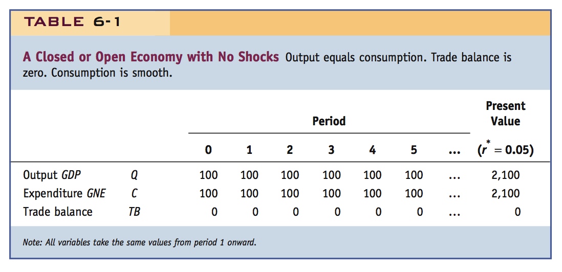
If this economy were open rather than closed, nothing would be different. The LRBC is satisfied because there is a zero trade balance at all times. Consumption C is perfectly smooth: every year the country consumes all 100 units of its output, and this is the country’s preferred consumption path. There are no gains from financial globalization because this open country prefers to consume only what it produces each year, and thus has no need to borrow or lend to achieve its preferred consumption path.
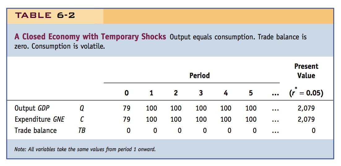
Closed Versus Open Economy: Shocks The smooth path for the closed economy cannot be maintained if it suffers shocks to output, such as one of the hurricanes discussed at the start of the chapter. Suppose there is a temporary unanticipated output shock of −21 units in year 0. Output Q falls to 79 in year 0 and then returns to a level of 100 thereafter. The change in the present value of output is the drop of 21 in year 0. The present value of output falls from 2,100 to 2,079, a drop of 1%.
Over time, will consumption in an open economy respond to this shock in the same way closed-economy consumption does? In the closed economy, there is no doubt what happens. Because all output is consumed and there is no possibility of a trade imbalance, consumption necessarily falls to 79 in year 0 and then rises back to 100 in year 1 and stays there forever. The path of consumption is no longer smooth, as shown in Table 6-2.
In the open economy, however, a smooth consumption path is still attainable because the country can borrow from abroad in year 0, and then repay over time. The country can’t afford its original smooth consumption path of 100 every period, because the present value of output is now less. So what smooth consumption path can it afford?
215
In the first section of this chapter, we spent some time deriving the LRBC. Now we can see why: the LRBC, given by Equation (6-4), is the key to determining a smooth consumption path in the face of economic shocks. Once we establish the present value of output, we know the present value of consumption, because these must be the same; from this fact we can figure out how to smooth consumption.
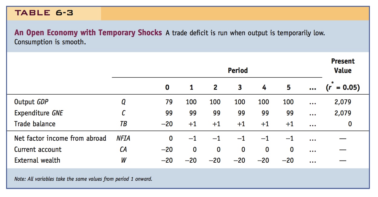
In this example, the present value of output Q has fallen 1% (from 2,100 to 2,079), so the present value of consumption must also fall by 1%. How should the country achieve this? Consumption can remain smooth, and satisfy the LRBC, if it falls by 1% (from 100 to 99) in every year. To double-check this logic, we compute the present value of C, using the perpetual loan formula again: 99 + 99/0.05 = 99 + 1,980 = 2,079. Because the present value of C and the present value of Q are equal, the LRBC is satisfied.
Table 6-3 shows the path of all the important macroeconomic aggregates for the open economy. In year 0, the country runs a trade balance of TB = −20 (a deficit), because output Q is 79 and consumption C is 99. In subsequent years, when output is 100, the country keeps consumption at 99, and has a trade balance TB = +1 (a surplus). Offsetting this +1 trade balance, the country must make net factor payments NFIA = −1 in the form of interest paid. The country must borrow 20 in year 0, and then make, in perpetuity, 5% interest payments of 1 unit on the 20 units borrowed.
216
In year 0, the current account CA (= TB + NFIA) is −20. In all subsequent years, net factor income from abroad is −1 and the trade balance is +1, implying that the current account is 0, with no further borrowing. The country’s external wealth W is therefore −20 in all periods, corresponding to the perpetual loan taken out in year 0. External wealth is constant at −20; it does not explode because interest payments are made in full each period and no further borrowing is required.
The lesson is clear. When output fluctuates, a closed economy cannot smooth consumption, but an open one can.
Generalizing The lesson of our numerical example applies to any situation in which a country wants to smooth its consumption when confronted with shocks. Suppose, more generally, that output Q and consumption C are initially stable at some value with Q = C and external wealth of zero. The LRBC is satisfied because the trade balance is zero at all times.
Now suppose output unexpectedly falls in year 0 by an amount ΔQ, and then returns to its prior value for all future periods. The loss of output in year 0 reduces the present value of output (GDP) by the amount ΔQ. To meet the LRBC, the country must lower the present value of consumption by the same amount. A closed economy accomplishes this by lowering its consumption by the whole amount of ΔQ in year 0. That is its only option! An open economy, however, lowers its consumption uniformly (every period) by a smaller amount, ΔC < ΔQ. But how big a reduction is needed to meet the LRBC?
Because consumption falls less than output in year 0, the country will run a trade deficit of ΔQ − ΔC < 0 in year 0. The country must borrow from other nations an amount equal to this trade deficit, and external wealth falls by the amount of that new debt. In subsequent years, output returns to its normal level but consumption stays at its reduced level, so trade surpluses of ΔC are run in all subsequent years.
Do a temporary decrease in income in the two-period Fisher model.
Because the LRBC requires that these surpluses be large enough to service the debt, we know how large the drop in consumption must be. A loan of ΔQ − ΔC in year 0 requires interest payments of r*(ΔQ − ΔC) in later years. If the subsequent trade surpluses of ΔC are to cover these interest payments, then we know that ΔC must be chosen so that
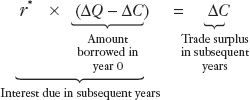
To find out how big a cut in consumption is necessary, we rearrange and find that
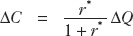
Note that the fraction in the above equation is between zero and 1. Thus, the generalized lesson is that an open economy only needs to lower its steady consumption level by a fraction of the size of the temporary output loss. [For instance, in the previous numerical example, ΔC = (0.05/1.05) × (21) = 1, so consumption had to fall by 1 unit.]
Smoothing Consumption When a Shock Is Permanent We just showed how an open economy uses international borrowing to smooth consumption in response to a temporary shock to output. When the shock is permanent, however, the outcome is different. With a permanent shock, output will be lower by ΔQ in all years, so the only way either a closed or open economy can satisfy the LRBC while keeping consumption smooth is to cut consumption by ΔC = ΔQ in all years. This is optimal, even in an open economy, because consumption remains smooth, although at a reduced level.
217
Now do a permanent shock in the two-period model and show that CA need not change at all.
Comparing the results for a temporary shock and a permanent shock, we see an important point: consumers can smooth out temporary shocks—they have to adjust a bit, but the adjustment is far smaller than the shock itself—but they must adjust immediately and fully to permanent shocks. For example, if your income drops by 50% just this month, you might borrow to make it through this month with minimal adjustment in spending; however, if your income is going to remain 50% lower in every subsequent month, then you need to cut your spending permanently.
Summary: Save for a Rainy Day
A simple phrase, but it helps fix the idea.
Financial openness allows countries to “save for a rainy day.” This section’s lesson has a simple household analogy. If you cannot use financial institutions to lend (save) or borrow (dissave), you have to spend what you earn each period. If you have unusually low income, you have little to spend. If you have a windfall, you have to spend it all. Borrowing and lending to smooth consumption fluctuations makes a household better off. The same applies to countries.
In a closed economy, consumption must equal output in every period, so output fluctuations immediately generate consumption fluctuations. In an open economy, the desired smooth consumption path can be achieved by running a trade deficit during bad times and a trade surplus during good times. By extension, deficits and surpluses can also be used to finance extraordinary and temporary emergency spending needs, such as the costs of war (see Side Bar: Wars and the Current Account).
Add government expenditures and taxes to the two-period model. Then a war is like a temporary decline in the endowment and creates a CA deficit. You also demonstrate the Ricardian argument that a tax cut would have no affect on the CA.
Wars are canonical examples of temporary adverse shocks. Countries often borrow in wartime, and run CA deficits.
Wars and the Current Account
Our theory of consumption smoothing can take into account temporary and “desired” consumption shocks. The most obvious example of such a shock is war.
Although we assumed zero government spending above, in reality, countries’ consumption includes private consumption C and public consumption G. It is simple to augment the model to include G as well as C. Under this circumstance, the constraint is that the present value of GNE (C + G) must equal the present value of GDP. A war means a temporary increase in G.
Borrowing internationally to finance war-related costs goes back centuries. Historians have long argued about the importance of the creation of the British public debt market as a factor in the country’s rise to global leadership compared with powerful continental rivals like France. From the early 1700s (which saw rapid financial development led by major financiers like the Rothschilds) to the end of the Napoleonic Wars in 1815, the British were able to maintain good credit; they could borrow domestically and externally cheaply and easily (often from the Dutch) to finance the simultaneous needs of capital formation for the Industrial Revolution and high levels of military spending.
In the nineteenth century, borrowing to finance war-related costs became more commonplace. In the 1870s, the defeated French issued bonds in London to finance a reparation payment to the triumphant Germans. World War I and World War II saw massive lending by the United States to other Allied countries. More recently, when the United States went to war in Afghanistan (2001) and Iraq (2003), there was a sharp increase in the U.S. current account deficit and in external debt due in part to war-related borrowing.
218
They find this a little abstract, so take it step by step: Write down this ratio and interpret the standard deviations for them. Then tell an intuitive story for why perfect smoothing would make this ratio zero.
Emphasize that perfect smoothing is only possible if risks are idiosyncratic.
Does financial integration reduce consumption volatility? Consumption volatility should be higher in countries with capital controls than those without them. However, both types of countries exhibit similar, high consumption volatility relative to GDP volatility.
Consumption Volatility and Financial Openness
Does the evidence show that countries avoid consumption volatility by embracing financial globalization? A simple test might be to compute the ratio of consumption volatility to output volatility (where volatility equals the standard deviation of the growth rate). If consumption smoothing is achieved, the computed ratio ought to fall. In fact, in our simple model of a small, open economy that can borrow or lend without limit, and that prefers a perfectly smooth path of consumption, this ratio should fall to zero because the economy can take advantage of financial globalization by borrowing and lending to other countries. In practice, this ratio will not be zero if all countries are affected by common global shocks. For example, if every country suffers a negative shock, every country will want to borrow, but that will not be possible: if all countries want to borrow, no countries will want to lend. In practice, however, not all shocks are global, so countries ought to be able to achieve some reduction in consumption volatility through external finance. (We consider the importance of local and global shocks later in this chapter.)
With this in mind, Figure 6-5 presents some discouraging evidence. On the horizontal axis, countries are sorted into 10 groups (deciles) from those that participate least in financial globalization (are least financially liberalized) to those that participate most. On the left are least open countries with tight capital controls (generally poorer countries), on the right are the more open countries that permit free movement of capital (mostly advanced countries). For all these countries, we assess their ability to smooth total consumption (C + G) in the period from 1995 to 2004 using annual data. In closed countries, we would expect that the volatility of consumption would be similar to the volatility of output (GDP) so that the ratio of the two would be close to 100%. But if an open country were able to smooth consumption in line with our simple model, this ratio ought to be lower than 100%.
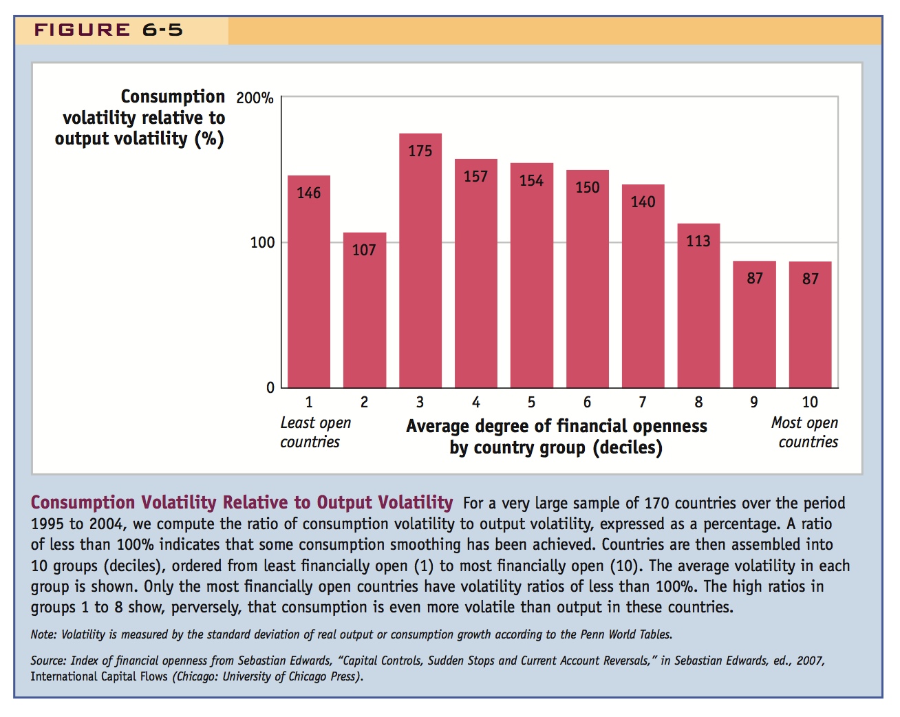
219
The figure shows that most groups of countries have an average consumption-to-output volatility ratio of well above 100%. Moreover, as financial liberalization increases, this ratio shows little sign of decrease until fairly high levels of liberalization are reached (around the seventh or eighth decile). Indeed, until we get to the ninth and tenth deciles, all of these ratios are above 100%.
Similar findings have been found using a variety of tests, and it appears that only at a very high level of financial liberalization does financial globalization deliver modest consumption-smoothing benefits.9
Why are these findings so far from the predictions of our model? In poorer countries, some of the relatively high consumption volatility must be unrelated to financial openness—it is there even in closed countries. In the real world, households are not identical and global capital markets do not reach every person. Some people and firms do not or cannot participate in even domestic financial markets, perhaps because of backward financial systems. Other problems may stem from the way financial markets operate (e.g., poor transparency and regulation) in emerging market countries that are partially open and/or have partially developed their financial systems.
The evidence may not imply a failure of financial globalization, but it does not provide a ringing endorsement either. Consumption-smoothing gains may prove elusive for emerging markets until they advance further by improving poor governance and weak institutions, developing their financial systems, and pursuing further financial liberalization.
Use this as an opening to talk about credit constraints in the two-period model, and emphasize they may be particularly binding for developing countries.
Highlight the interesting interaction of precautionary saving motives with credit constraints.
Suggest that this may be having important macroeconomic consequences, to which we will return much later in the book.
If poor countries anticipate facing credit constraints, they may respond to the presence of random shocks by engaging in precautionary saving, setting aside a buffer-stock of external reserves as a “rainy day” fund. Precautionary saving is common, and takes two forms: (1) The acquisition of foreign reserves by central banks, and (2) sovereign wealth funds, state owned asset-management funds that invest government savings.
Precautionary Saving, Reserves, and Sovereign Wealth Funds
One obstacle to consumption smoothing in poorer countries is the phenomenon of sudden stops, which we noted earlier. If poorer countries can’t count on credit lines to be there when they need them, they may fall back on an alternative strategy of engaging in precautionary saving, whereby the government acquires a buffer of external assets, a “rainy day fund.” That is, rather than allowing external wealth to fluctuate around an average of zero, with the country sometimes being in debt and sometimes being a creditor, the country maintains a higher positive “average balance” in its external wealth account to reduce or even eliminate the need to go into a net debt position. This approach is costly, because the country must sacrifice consumption to build up the buffer. However, poor countries may deem the cost to be worthwhile if it allows them to smooth consumption more reliably once the buffer is established.
In the world economy today, precautionary saving has been on the rise and it takes two forms. The first is the accumulation of foreign reserves by central banks. Foreign reserves are safe assets denominated in foreign currency, like U.S. Treasury securities and other low-risk debt issued by governments in rich, solvent countries. They can be used not only for precautionary saving but for other purposes, such as maintaining a fixed exchange rate. As external assets on the nation’s balance sheet, these reserves can be deployed during a sudden stop to cushion the blow to the domestic economy. Many economists argue that some part or even the greater part of reserve accumulation in recent years in emerging markets is driven by this precautionary motive.10
220
The second form of precautionary saving by governments is through what are called sovereign wealth funds, state-owned asset management companies that invest some government savings (possibly including central bank reserves) overseas. Often, the asset management companies place the government savings in safe assets; increasingly, however, the funds are being placed in riskier assets such as equity and FDI. Some countries, such as Norway (which had an oil boom in the 1970s), use such funds to save windfall gains from the exploitation of natural resources for future needs. Many newer funds have appeared in emerging markets and developing countries (such as Singapore, China, Malaysia, and Taiwan), but these funds have been driven more by precautionary saving than resource booms.
As of March 2013, the countries with the biggest sovereign wealth funds were China ($1.2 trillion), Abu Dhabi ($745 billion), Norway ($716 billion), and Saudi Arabia ($538 billion), with other large funds (more than $75 billion each) in Kuwait, Russia, Singapore, Qatar, Libya, and Australia.11
Most observers believe it is likely that sovereign wealth funds will continue to grow in size, and that their use will spread to other countries (see Headlines: Copper-Bottomed Insurance). It is interesting that, despite having a legitimate economic rationale, these funds may generate international tensions, as they already have, by attempting to acquire politically sensitive equity and FDI assets from advanced countries.