2 How Pegs Work: The Mechanics of a Fixed Exchange Rate

To start, we must first understand how a pegged exchange rate works. Once we know what policy makers have to do to make a peg work, we will then be in a position to understand the factors that make a peg break.

To help us understand the economic mechanisms that operate in a fixed exchange rate system, we develop a simple model of what a central bank does. We then use the model to look at the demands placed on a central bank when a country adopts a fixed exchange rate.

Preliminaries and Assumptions

We consider a small open economy, in which the authorities are trying to peg to some foreign currency. We make the following assumptions, some of which may be relaxed in later analyses:

• For convenience, and without implying that we are referring to any specific country, we assume that the home currency is called the peso. The currency to which home pegs is the U.S. dollar. We assume the authorities have been maintaining a fixed exchange rate, with E fixed at = 1 (one peso per U.S. dollar).
• The country’s central bank controls the money supply M by buying and selling assets in exchange for cash. The central bank trades only two types of assets: domestic bonds, often government bonds, denominated in local currency (pesos), and foreign assets, denominated in foreign currency (dollars).
• The central bank intervenes in the forex market to peg the exchange rate. It stands ready to buy and sell foreign exchange reserves at the fixed exchange rate . If it has no reserves, it cannot do this and the exchange rate is free to float: the peg is broken.
• Unless stated otherwise, we assume that the peg is credible: everyone believes it will continue to hold. Uncovered interest parity then implies that the home and foreign interest rates are equal: i = i*.
• We also assume for now that the economy’s level of output or income is assumed to be exogenous; that is, it is treated as given and denoted Y.
• There is a stable foreign price level P* = 1 at all times. In the short run, the home country’s price is sticky and fixed at a level P = 1. In the long run, if the exchange rate is kept fixed at 1, then the home price level will be fixed at 1 as a result of purchasing power parity.
• As in previous chapters, the home country’s demand for real money balances M/P is determined by the level of output Y and the nominal interest rate i and takes the usual form, M/P = L(i)Y. The money market must be in equilibrium, so money demand is always equal to money supply.
• We use the simplest model of a fixed exchange rate, where there is no financial system. The only money is currency, also known as M0 or the monetary base. The monetary base (M0) and broad money (M1) are then the same, so the money supply is denoted M. This assumption allows us to examine the operation of a fixed exchange rate system by considering only the effects of the actions of a central bank.
• If there is no financial system, we do not need to worry about the role of private banks in creating broad money through checking deposits, loans, and so on. A simple generalization would allow for banks by letting broad money be a constant multiple of the currency.6 Still, the existence of a banking system is important, and even without formal theory, we will see later in the chapter how it affects the operation of a fixed exchange rate.

The Central Bank Balance Sheet

To understand how the home central bank maintains the peg, we must understand how the home central bank manages its assets in relation to its sole liability, the money in circulation.

Suppose the central bank has purchased a quantity B pesos of domestic bonds. By, in effect, loaning money to the domestic economy, the central bank’s purchases are usually referred to as domestic credit created by the central bank. These purchases are also called the bank’s domestic assets. Because the central bank purchases these assets with money, this purchase generates part of the money supply. The part of the home money supply created as a result of the central bank’s issuing of domestic credit is denoted B.

Now suppose the central bank has also purchased a quantity R dollars of foreign exchange reserves, usually referred to as reserves or foreign assets, and that the exchange rate is pegged at a level = 1. The central bank also purchases its reserves with money. Thus, given that the exchange rate has always been 1 (by assumption), the part of the money supply created as a result of the central bank’s purchase of foreign exchange reserves is .7

Because the central bank holds only two types of assets, the last two expressions add up to the total money supply in the home economy:

This equation states that the money supply equals domestic credit plus reserves.

This expression is also useful when expressed not in levels but in changes:

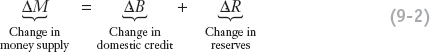
This expression says that changes in the money supply must result from either changes in domestic credit or changes in reserves.

For example, if the central bank buys additional reserves ΔR = 1,000 dollars, then the money it spends adds ΔM = 1,000 pesos to the money in circulation. If the central bank creates additional domestic credit of ΔB = 1,000 pesos, then it buys 1,000 pesos of government debt, and this also adds ΔM = 1,000 pesos to the money in circulation.

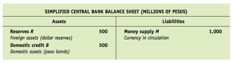
One common way of depicting Equation (9-1) is to write down each entry and construct the central bank balance sheet. The domestic debt and foreign reserves purchased by the central bank are its assets, B + R. The money supply issued by the central bank M is its liabilities.

Following is a hypothetical central bank balance sheet. The central bank has purchased 500 million pesos in domestic government bonds and 500 million pesos in foreign exchange reserves. The total money in circulation resulting from these purchases is 1,000 million pesos. As on any balance sheet, total assets equal total liabilities.

Fixing, Floating, and the Role of Reserves

The crucial assumption in our simple model is that the central bank maintains the peg by intervening in the foreign exchange market by buying and selling reserves at the fixed exchange rate. In other words, our model supposes that if the central bank wants to fix the exchange rate, it must have some reserves it can trade to achieve that goal. We also assume, for now, that it holds reserves only for this purpose. Thus:

We are assuming that the exchange rate is fixed if and only if the central bank holds reserves; and the exchange rate is floating if and only if the central bank has no reserves.

These assumptions simplify our analysis by clarifying the relationship between the central bank balance sheet and the exchange rate regime. In reality, the relationship may be less clear, but the mechanisms in our model still play a dominant role.

For example, countries may adjust domestic credit as well as reserves, but they never try to maintain a peg by relying solely on domestic credit adjustments and zero reserves. Why? In the very short run, forex market conditions can change so quickly that only direct intervention in that market through reserve trading can maintain the peg. In addition, large adjustments to domestic credit may pose problems in an emerging market by causing instability in the bond market as the central bank buys or sells potentially large amounts of government bonds.

Countries can also float and yet keep some reserves on hand for reasons that we ignore in our model so as to keep it simple. They may want reserves on hand for future emergencies, such as war; or as a savings buffer in the event of a sudden stop to financial flows; or so they can peg at some later date.8 Thus, the minimum level of reserves the central bank will tolerate on its balance sheet may not be at zero, but allowing for some other forms of reserves would not affect our analysis.

How Reserves Adjust to Maintain the Peg

We now turn to the key questions we need to answer to understand how a peg works. What level of reserves must the central bank have to maintain the peg? And how are reserves affected by changing macroeconomic conditions? If the central bank can maintain a level of reserves above zero, we know the peg will hold. If not, the peg breaks.

We can rearrange Equation (9-1) to solve for the level of reserves, with R = M − B. Why do we do that? It is important to remember that reserves are the unknown variable here: by assumption, reserves change as a result of the central bank’s interventions in the forex market, which it must undertake to maintain the peg.

Because (in nominal terms) money supply equals money demand, given by , we can restate and rearrange Equation (9-1) to solve for the level of reserves:

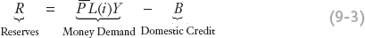
By substituting money demand for money supply, we can investigate how shocks to money demand (say, due to changes in output or the interest rate) or shocks to domestic credit affect the level of reserves.

We can solve this equation. Under our current assumptions, every element on the right-hand side is exogenous and known. The home price level is fixed, the output level is exogenous, interest parity tells us that the home interest rate equals the foreign interest rate, and we can treat domestic credit as predetermined by the central bank’s purchases of domestic government debt.

Why is this answer for the reserve level correct and unique? Recall how forex market equilibrium is attained from the chapter on exchange rates in the short run. If the central bank bought more reserves than this, home money supply would expand and the home nominal interest rate would fall, the peso would depreciate, and the peg would break. To prevent this, the central bank would need to intervene in the forex market. The central bank would have to offset its initial purchase of reserves to keep the supply of pesos constant and keep the exchange rate holding steady. Similarly, if the central bank sells reserves for pesos, it would cause the peso to appreciate and would have to reverse course and buy back the reserves. The peg means that the central bank must keep the reserves at the level specified in Equation (9-3).

Graphical Analysis of the Central Bank Balance Sheet

Based on this toolkit, we show the mechanics of a pegged exchange rate in Figure 9-4, which illustrates the central bank balance sheet. On the horizontal axis is the money supply M and on the vertical axis is domestic credit B, both measured in pesos. Money demand is initially at the level M₁, and domestic credit is at B₁.

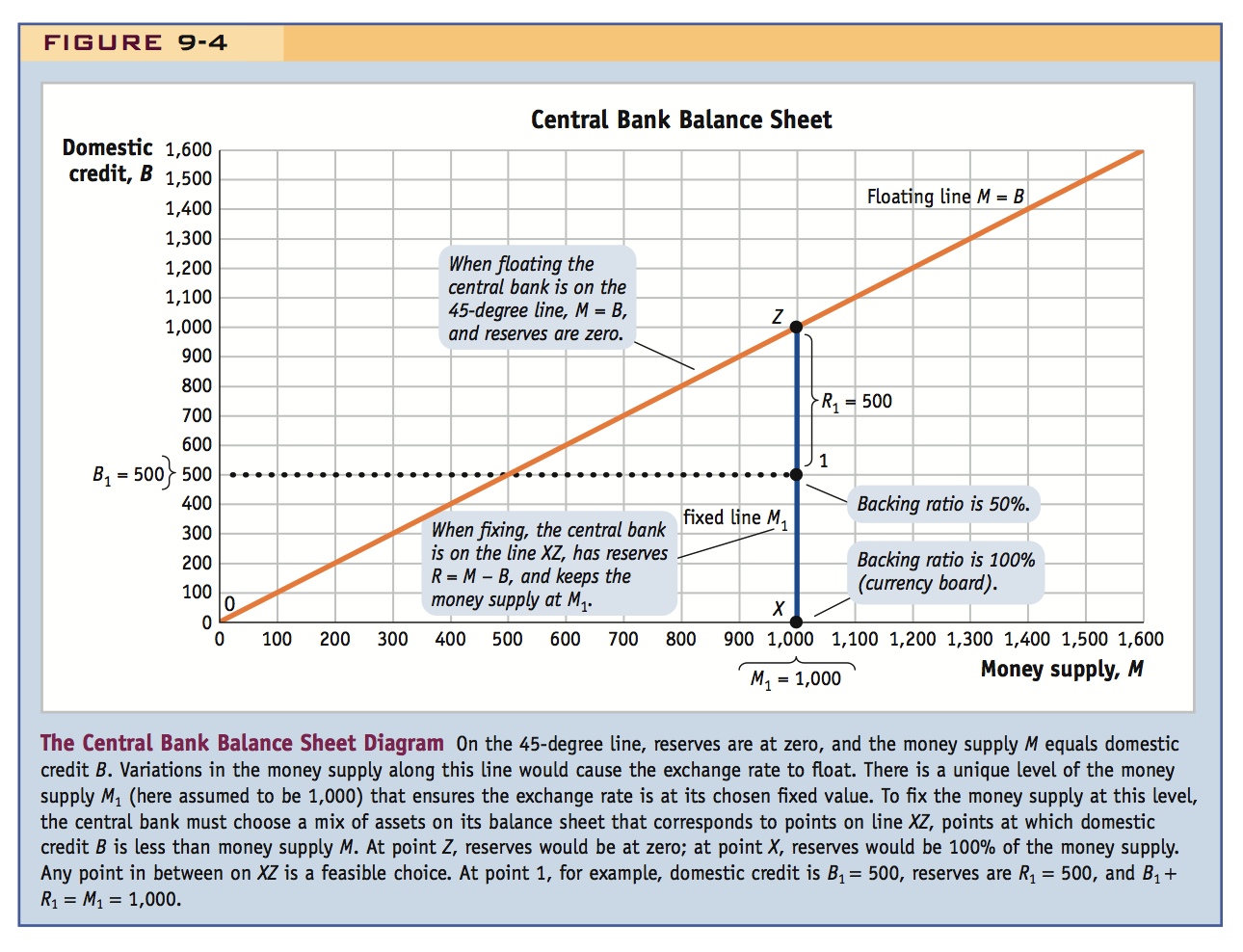
Two important lines appear in this figure. If reserves R are zero, then all of the money supply is due to domestic credit and Equation (9-1) tells us that M = B. The points where M = B are on the 45-degree line. Points on this line, like point Z, correspond to cases in which the central bank balance sheet contains no reserves. By assumption, the country will then have a floating exchange rate, so we call this the floating line.

When the assets of the central bank include both reserves and domestic credit, then B and R are both greater than zero and they add up to M. The state of the central bank balance sheet must correspond to a point such as point 1 in this diagram, somewhere on the vertical line XZ. We call this the fixed line because on this line the money supply is at the level M₃ necessary to maintain the peg.

If domestic credit is B₁, then reserves are R₁ = M₁ − B₁, the vertical (or horizontal) distance between point 1 and the 45-degree floating line. Hence, the distance to the floating line tells us how close to danger the peg is by showing how close the central bank is to the point at which reserves run out.9 The point farthest from danger is X, on the horizontal axis. At this point, domestic credit B is zero and reserves R equal the money supply M. A fixed exchange rate that always operates with reserves equal to 100% of the money supply is known as a currency board system.10

To sum up: if the exchange rate is floating, the central bank balance sheet must correspond to points on the 45-degree floating line; if the exchange rate is fixed, the central bank balance sheet must correspond to points on the vertical fixed line.

The model is now complete, and with the aid of our key tools—the tables and graphs of the central bank balance sheet—we can see how a central bank that is trying to maintain a peg reacts to two types of shocks. We first look at shocks to the level of money demand and then shocks to the composition of money supply.

Defending the Peg I: Changes in the Level of Money Demand

We first look at shocks to money demand and how they affect reserves by altering the level of money supply M. As we saw in Equation (9-3), money supply is equal to money demand, as given by the equation . If the price level is fixed, then money demand will fluctuate only in response to shocks in output Y and the home interest rate i (which equals the foreign interest rate i* if the peg is credible). For now, output is exogenous, and a rise in output will raise money demand. The foreign interest rate is also exogenous, and a rise in the foreign interest rate will raise the home interest rate and thus lower money demand. We assume all else is equal, so domestic credit is constant.

A Shock to Home Output or the Foreign Interest Rate Suppose output falls or the foreign interest rate rises. We treat either of these events as an exogenous shock for now, all else equal, and suppose it decreases money demand by, say, 10% at the current interest rate.

For example, suppose we start with a central bank balance sheet as given earlier. Initially, money supply is M₁ = 1,000 million pesos. Suppose money demand then falls by 10%. This would lower money demand by 10% to M₂ = 900 million pesos. A fall in the demand for money would lower the interest rate in the money market and put depreciation pressure on the home currency. A floating exchange rate would allow the home currency to depreciate in these circumstances. To maintain the peg, the central bank must keep the interest rate unchanged. To achieve this goal, it must sell 100 million pesos ($100 million) of reserves, in exchange for cash, so that money supply contracts as much as money demand. The central bank’s balance sheet will then be as follows:

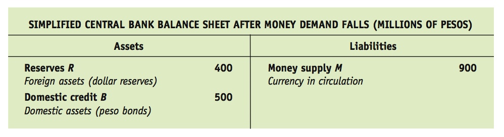
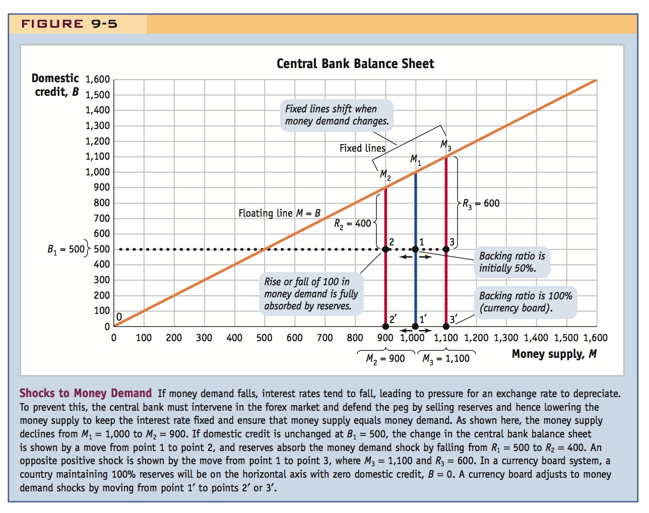
In Figure 9-5, we can trace the implications of the shock in a graph. The demand for money has fallen, so the fixed line is still vertical, but it shifts from the initial money demand level M₁ = 1,000 to a new lower level M₂ = 900. There is no change to domestic credit, so it remains constant at the level B₁ = 500. Thus, the central bank’s balance sheet position shifts from point 1 to point 2. This shift takes the balance sheet position closer to the floating line in the diagram: reserves are falling. At point 2, reserves have fallen from R₁ = 500 to R₂ = 400, as shown.

Figure 9-5 also shows what would happen with the opposite shock. If money demand increased by 10% from the initial money demand level M₁ = 1,000 to a new higher level M₃ = 1,100, the central bank would need to prevent an interest rate rise and an appreciation by expanding the money supply by 100 pesos. The central bank would need to intervene and increase the money supply by purchasing $100 of reserves. The central bank’s balance sheet position would then shift from point 1 to point 3, moving away from the floating line, with reserves rising from R₁ = 500 to R₃ = 600.

Equation (9-3) confirms these outcomes as a general result when domestic credit is constant (at B₁ in our example). We know that if the change in domestic credit is zero, ΔB = 0, then any change in money supply must equal the change in reserves, ΔR = ΔM. This is also clear from Equation (9-2).

We have shown the following: holding domestic credit constant, a change in money demand leads to an equal change in reserves.

The Importance of the Backing Ratio In the first example above, money demand and money supply fell by 10% from 1,000 to 900, but reserves fell by 20% from 500 to 400. The proportional fall in reserves was greater than the proportional fall in money because reserves R were initially only 500 and just a fraction (one-half) of the money supply M, which was 1,000. When money demand fell by 100, reserves had to absorb all of the change, with domestic credit unchanged.

The ratio R/M is called the backing ratio, and it indicates the fraction of the money supply that is backed by reserves on the central bank balance sheet. It, therefore, tells us the size of the maximum negative money demand shock that the regime can withstand without running out of reserves if domestic credit remains unchanged. In our example, the backing ratio was 0.5 or 50% (reserves were 500 and money supply 1,000 initially), so the central bank could absorb up to a 50% decline in the money supply before all of its reserves run out. Because reserves were only 500 to start with, a shock of −500 to money demand would cause reserves to just run out.

In general, for a given size of a shock to money demand, a higher backing ratio will better insulate an economy against running out of reserves, all else equal.11

In Figure 9-5, the higher the backing ratio, the higher the level of reserves R and the lower the level of domestic credit B, for a given level of money supply M. In other words, the central bank balance sheet position on this figure would be closer to the horizontal axis and farther away from the floating line. This is a graphical illustration of the idea that a high backing ratio makes a peg safer.

Currency Board Operation This maximum backing ratio of 100% is maintained at all times by a currency board. A 100% backing ratio puts the country exactly on the horizontal axis. In Figure 9-5, a currency board would start at point 1′, not point 1. Because reserves would then be 1,000 to start with, a shock of up to −1,000 to money demand could be accommodated without reserves running out. In the face of smaller shocks to money demand such as we have considered, of plus or minus 100, the central bank balance sheet would move to points 2′ or 3′, with reserves equal to money supply equal to money demand equal to 900 or 1,100. These points are as far away from the 45-degree floating line as one can get in this diagram, and they show how a currency board keeps reserves at a maximum 100%. A currency board can be thought of as the safest configuration of the central bank’s balance sheet because with 100% backing, the central bank can cope with any shock to money demand without running out of reserves. Currency boards are considered a hard peg because their high backing ratio ought to confer on them greater resilience in the face of money demand shocks.

Why Does the Level of Money Demand Fluctuate? Our result tells us that to maintain the fixed exchange rate, the central bank must have enough reserves to endure a money demand shock without running out. A shock to money demand is not under the control of the authorities, but they must respond to it. Thus, it is important for policy makers to understand the sources and likely magnitudes of such shocks. Under our assumptions, money demand shocks originate either in shocks to home output Y or the foreign interest rate i* (because under a credible peg i = i*).

We have studied output fluctuations in earlier chapters, and one thing we observed was that output tends to be much more volatile in emerging markets and developing countries. Thus, the prudent level of reserves is likely to be much higher in these countries. Volatility in foreign interest rates can also be important, whether in U.S. dollars or in other currencies that form the base for pegs.

However, we must also confront a new possibility—that the peg is not fully credible and that simple interest parity fails to hold. In this case, the home interest rate will no longer equal the foreign interest rate, and additional disturbances to home money demand can be caused by the spread between the two. As we now see, this is a vital step toward understanding crises in emerging markets and developing countries.

Risk Premiums in Advanced and Emerging Markets

So far in the book, we have assumed that uncovered interest parity (UIP) requires that the domestic return (the interest rate on home bank deposits) equals the foreign interest rate plus the expected rate of depreciation of the home currency. However, an important extension of UIP needs to be made when additional risks affect home bank deposits: a risk premium is then added to the foreign interest rate to compensate investors for the perceived risk of holding a home domestic currency deposit. This perceived risk is due to an aversion to exchange rate risk or a concern about default risk:

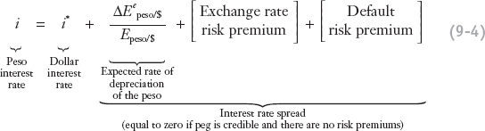
The left-hand side is still the domestic return, but the right-hand side is now a risk-adjusted foreign return. The final three terms are the difference between home and foreign interest rates, and their sum total is known as the interest rate spread. What causes these spreads?

The first part of the interest rate spread is the currency premium:

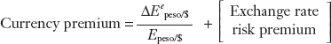
The currency premium should be zero for a credibly pegged exchange rate: the peso is not expected to change in value relative to the dollar. But if a peg is not credible, and investors suspect that the peg may break, there could be a premium reflecting both the size of the expected depreciation and the currency’s perceived riskiness. The currency premium therefore reflects the credibility of monetary policy.

The second part of the interest rate spread is known as the country premium:

The country premium is compensation for perceived default risk (settlement or counterparty risk). It will be greater than zero if investors suspect a risk of losses when they attempt to convert a home (peso) asset back to foreign currency (dollars) in the future. Such a loss might occur because of expropriation, bank failure, surprise taxation, delays, capital controls, other regulations, and so on. The country premium therefore reflects the credibility of property rights.

363

Why does all this matter? Fluctuations in currency and country premiums have the same effect in Equation (9-4) as fluctuations in the foreign interest rate i*. Sudden increases in the interest rate spread raise the risk-adjusted foreign return and imply sudden increases in the domestic return, here given by the (peso) interest rate i. In some countries, these spreads can be large and volatile—and even more volatile than the foreign interest rate.

Figure 9-6 presents interest rate spreads for two countries with fixed exchange rates. Panel (a) shows an advanced country, Denmark, which pegs to the euro; panel (b) shows an emerging market, Argentina, which pegged to the dollar from 1991 to 2001.

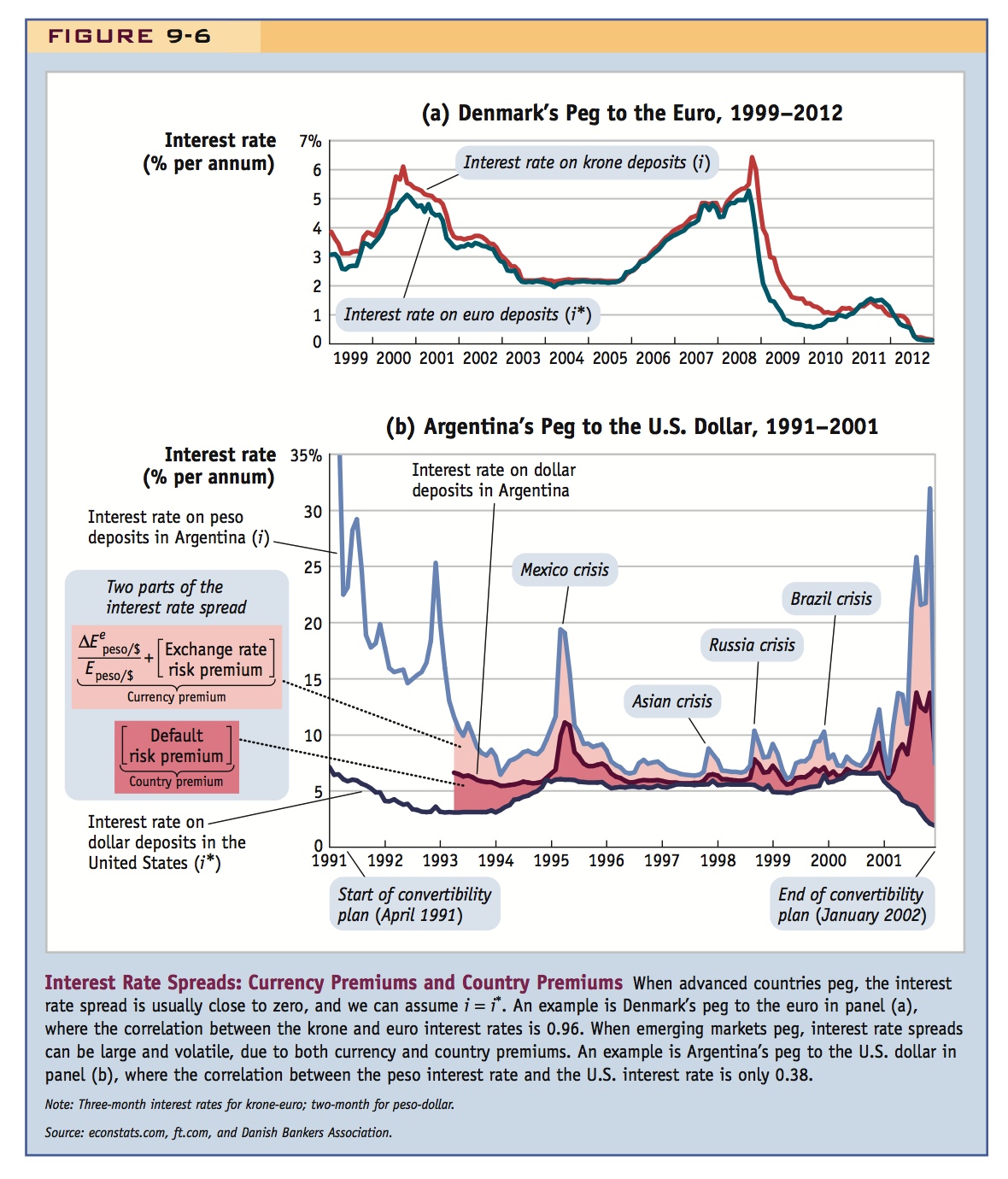
In Denmark, there was some spread in the early years of the euro from 1999 to 2002 (up to about 0.5% per year), and again some wider spreads in the 2009–10 crisis period, perhaps reflecting a worry that the krone-euro peg might not endure. Otherwise the spread was almost imperceptible (less than 0.1% per year). Overall, the simple correlation between the krone interest rate and the euro interest rate was very high, equal to 0.96. Investors came to see the peg as credible, eliminating the currency premium almost entirely. They also had no fear of default risk if they invested in Denmark, eliminating the country premium almost entirely. Thus one could assume at most times that i was approximately equal to i* with no spread.

In Argentina the spreads were large: note the bigger vertical scale in panel (b). The annual peso and dollar interest rates were far apart, often differing by 2 or 3 percentage points and sometimes differing by more than 10 percentage points. Most striking is that changes in the spread were usually more important in determining the Argentine interest rate than were changes in the actual foreign (U.S. dollar) interest rate. Overall, the correlation between the peso interest rate i and the dollar interest rate i* was low, equal to only 0.38. What was going on?

We can separately track currency risk and country risk because Argentine banks offered interest-bearing bank deposits denominated in both U.S. dollars and Argentine pesos. The lower two lines in panel (b) show the interest rate on U.S. dollar deposits in the United States (i*) and the interest rate on U.S. dollar deposits in Argentina. Because the rates are expressed in the same currency, the difference between these two interest rates cannot be the result of a currency premium. It represents a pure measure of country premium: investors required a higher interest rate on dollar deposits in Argentina than on dollar deposits in the United States because they perceived that Argentine deposits might be subject to a default risk. (Investors were eventually proved right: in the 2001–2002 crisis, many Argentine banks faced insolvency, some were closed for a time, capital controls were imposed at the border, and a “pesification” law turned many dollar assets into peso assets ex post, a form of expropriation and a contractual default.)

The upper line in panel (b) shows the interest rate on peso deposits in Argentina (i), which is even higher than the interest rate on U.S. dollar deposits in Argentina. Because these are interest rates on bank deposits in the same country, the difference between these two rates cannot be due to a country premium. It represents a pure measure of currency premium. Investors required a higher interest rate on peso deposits in Argentina than on dollar deposits in Argentina because they perceived that peso deposits might be subject to a risk of depreciation, that is, a collapse of the peg. (Investors were eventually proved right again: in the 2001–2002 crisis, the peso depreciated by 75% from $1 to the peso to about $0.25 to the peso, or four pesos per U.S. dollar.)

364

Summary Pegs in emerging markets are different from those in advanced countries. Because of fluctuations in interest rate spreads, they are subject to even greater interest rate shocks than the pegs of advanced countries, as a result of credibility problems. Currency premiums may fluctuate due to changes in investors’ beliefs about the durability of the peg, a problem of the credibility of monetary policy. Country premiums may fluctuate due to changes in investors’ beliefs about the security of their investments, a problem of the credibility of property rights.

365

Still, not every movement in emerging market spreads is driven by economic fundamentals. For example, in Argentina the figure shows that investors revised their risk premiums sharply upward when other emerging market countries were experiencing crises in the 1990s: Mexico in 1994, Asia in 1997, and later Russia and Brazil. With the exception of Brazil (a major trade partner for Argentina), there were no major changes in Argentine fundamentals during these crises. Thus, many economists consider this to be evidence of contagion in global capital markets, possibly even a sign of market inefficiency or irrationality, where crises in some parts of the global capital markets trigger adverse changes in market sentiment in faraway places.

The Argentine Convertibility Plan Before the Tequila Crisis

The central bank balance sheet diagram helps us to see how a central bank manages a fixed exchange rate and what adjustments it needs to make in response to a shock in money demand.

We can put this analysis to use with a concrete example: the operation of Argentina’s fixed exchange rate system (known as the Convertibility Plan), which began in 1991 and ended in 2002. In this plan, a peg was maintained as one peso per dollar. With the aid of Figure 9-7, we focus first on how the central bank managed its balance sheet during an early phase of the plan, in 1993 and 1994. (We will discuss later years shortly.)

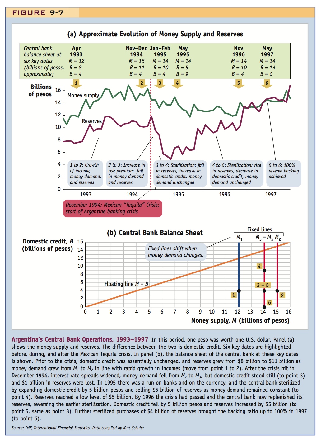
Money Demand Shocks, 1993–1994 The evolution of money supply and reserves is shown in panel (a). From point 1 to point 2 (April 1993 to November/December 1994), all was going well. Argentina had recovered from its hyperinflation in 1989 to 1990, prices were stable, the economy was growing, and so was money demand. Because money demand must equal money supply, the central bank had to increase the money supply. The central bank kept domestic credit more or less unchanged in this period at 4 billion pesos, so reserves had to expand (from 8 billion to 11 billion pesos) as the base money supply expanded (from 12 billion to 15 billion pesos). The backing ratio rose from about 67% (8/12) to about 73% (11/15). In the central bank balance sheet diagram in panel (b), this change is shown by the horizontal move from point 1 to point 2 as the money demand shock causes the fixed line to shift out from M₁ to M₂, so that higher levels of base money supply are now consistent with the peg.

Then an unexpected nasty shock happened: a risk premium shock occurred as a result of the so-called Tequila crisis in Mexico in December 1994. Interest rate spreads widened for Argentina because of currency and country premiums, raising the home interest rate. Argentina’s money demand fell. In panel (a), from point 2 to point 3 (November/December 1994 to January/February 1995), base money supply contracted by 1 billion pesos, and this was absorbed almost entirely by a contraction in reserves from 11 billion to 10 billion pesos. The backing ratio fell to about 71% (10/14). In panel (b), this change is shown by the horizontal move from point 2 to point 3 as the money demand shock causes the fixed line to shift in from M₂ to M₃.

366

367

To Be Continued Through all of these events, the backing ratio remained high and domestic credit remained roughly steady at around 4 billion pesos, corresponding to our model’s assumptions so far. People wanted to swap some pesos for dollars, but nothing catastrophic had happened. However, this was about to change. The shock to Argentina’s interest rate proved damaging to the real economy and especially the banking sector. Argentines also became nervous about holding pesos. Foreigners stopped lending to Argentina as the economic situation looked riskier. The central bank stepped in to provide assistance to the ailing banks. But we have yet to work out how a central bank can do this and still maintain a peg. After we complete that task, we will return to the story and see how Argentina managed to survive the Tequila crisis.

Defending the Peg II: Changes in the Composition of Money Supply

So far we have examined changes to the level of money demand. We have assumed that the central bank’s policy toward domestic credit was passive, and so B has been held constant up to now. In contrast, we now study shocks to domestic credit B, all else equal. To isolate the effects of changes in domestic credit, we assume that money demand is constant.

If money demand is constant, then so is money supply. Therefore, the key lesson of this section will be that, on its own, a change in domestic credit cannot affect the level of the money supply, it can only affect the composition in terms of domestic credit and reserves.

A Shock to Domestic Credit Suppose that the central bank increases domestic credit by an amount ΔB > 0 from B₁ to B₂. This increase could be the result of an open market operation by the bank’s bond trading desk to purchase bonds from private parties. Or it could be the result of a demand by the country’s economics ministry that the bank directly finance government borrowing. For now we will not concern ourselves with the cause of this policy decision, and will not discuss whether it makes any sense. We just ask what implications it has for a central bank trying to maintain a peg, all else equal. We assume that domestic output and the foreign interest rate are unchanged.

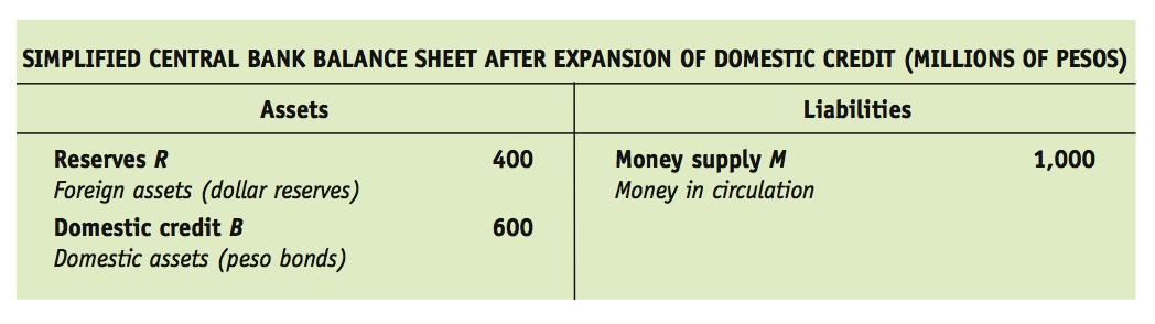
For example, suppose we start with a central bank balance sheet with money supply at its initial level of M₁ = 1,000 million pesos. The bank then expands domestic credit from $500 million pesos by buying ΔB = $100 million of peso bonds. All else equal, this action puts more money in circulation, which lowers the interest rate in the money market and puts depreciation pressure on the exchange rate. A floating rate would depreciate in these circumstances. To defend the peg, the central bank must sell enough reserves to keep the interest rate unchanged. To achieve that, it must sell 100 million pesos ($100 million) of reserves, in exchange for cash, so that the money supply remains unchanged. The central bank’s balance sheet will then be as follows:

What is the end result? Domestic credit B changes by +100 million pesos (rising to 600 million pesos), foreign exchange reserves R change by −100 million pesos (falling to 400 million pesos), and the money supply M remains unchanged (at 1,000 million pesos).

The bond purchases expand domestic credit but also cause the central bank to lose reserves as it is forced to intervene in the forex market. There is no change in monetary policy as measured by home money supply (or interest rates) because the sale and purchase actions by the central bank offset each other exactly. This type of central bank action is called sterilization, a sterilized intervention, or a sterilized sale of reserves.

In Figure 9-8, we show the implications of sterilization policies. On the vertical axis, domestic credit rises from B₁ to B₂. The balance sheet position of the central bank therefore shifts up the fixed line from point 1 to point 2. Reserves fall by ΔB from R₁ = $500 million to R₂ = $400 million. The central bank has moved closer to point Z, the danger point of zero reserves on the 45-degree line. The backing ratio falls from 50 to 40%.

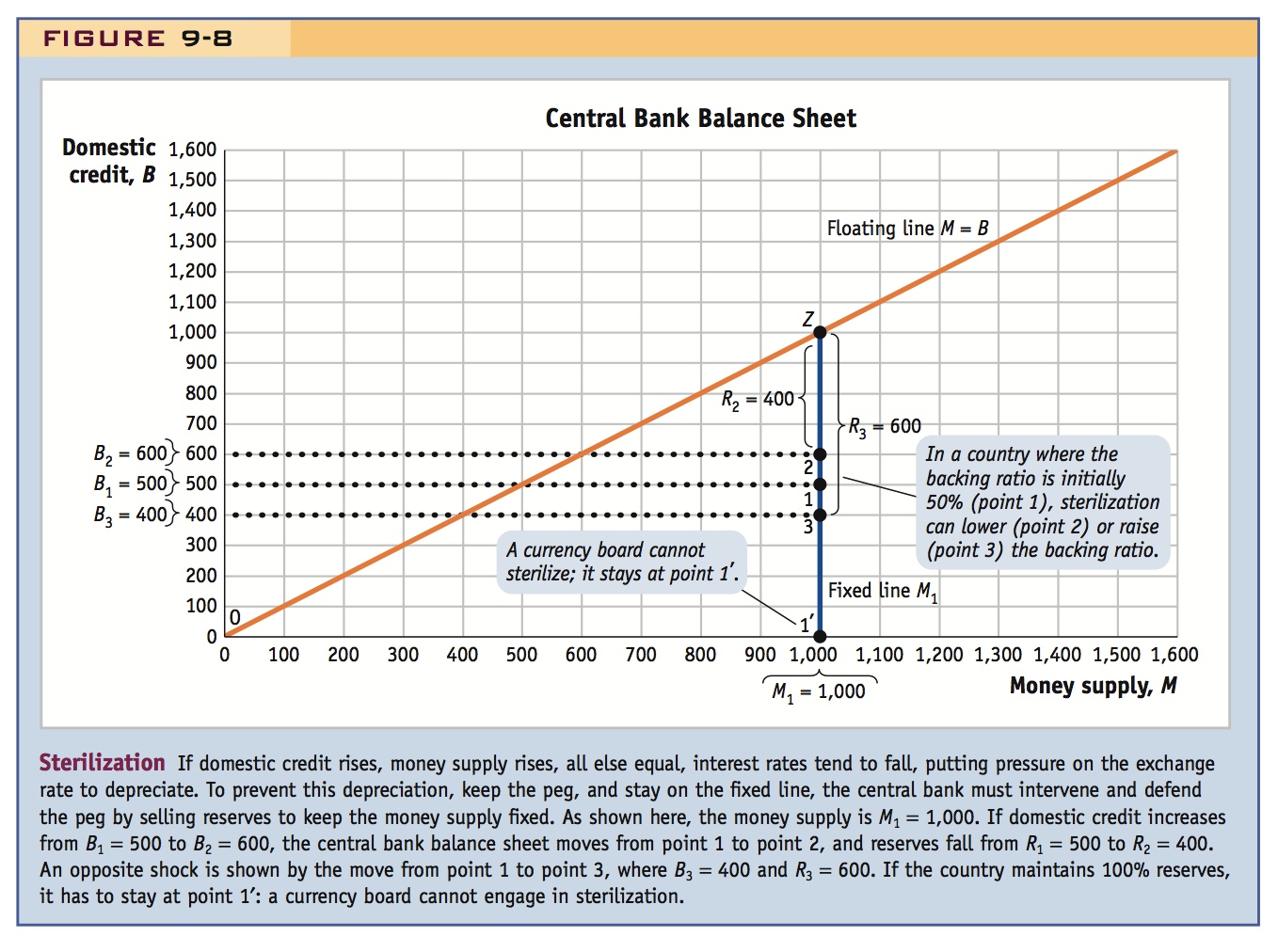
Figure 9-8 also shows what would happen with the opposite shock. If domestic credit fell by 100 million pesos to 400 million pesos at B₃, with an unchanged money demand, then reserves would rise by $100 million. The central bank’s balance sheet ends up at point 3. Reserves rise from R₁ = 500 to R₃ = 600. The backing ratio now rises from 50% to 60%.

We also see in Figure 9-8 that sterilization is impossible in the case of a currency board because a currency board requires that domestic credit always be zero and that reserves be 100% of the money supply at all times.

Equation (9-3) confirms this as a general result. We know that if the change in money demand is zero, then so is the change in money supply, ΔM = 0; hence, the change in domestic credit, ΔB > 0, must be offset by an equal and opposite change in reserves, ΔR = −ΔB < 0. This is also clear from Equation (9-2).

We have shown the following: holding money demand constant, a change in domestic credit leads to an equal and opposite change in reserves, which is called a sterilization.

Why Does the Composition of the Money Supply Fluctuate? Our model tells us that sterilization has no effect on the level of money supply and hence no effect on interest rates and the rest of the economy. This prompts a question: if sterilization has no effect on these variables, why would central banks bother to do it? In the case of buying and selling government bonds, which is the predominant form of domestic credit, the effects are controversial but are generally thought to be small. The only possible effect would be indirect, via portfolio changes in the bond market. If the central bank absorbs some government debt, it leaves less peso debt for the private sector to hold, and this could change the risk premium on the domestic interest rate. But evidence for that type of effect is rather weak.12

However, there is another type of domestic credit that can have very important effects on the wider economy. This is domestic credit caused by a decision by the central bank to lend to private commercial banks in difficulty. Here, the central bank would be fulfilling one of its traditional responsibilities as the protector of the domestic financial system. This action has real effects because a domestic banking crisis, if allowed to happen, can cause serious economic harm by damaging the economy’s payments system and credit markets.

In theory, when it comes to banks that are having difficulties, economists distinguish between banks that are illiquid and those that are insolvent. Let’s see how loans from the central bank to private commercial banks affect the central bank balance sheet for these two cases. Note that for these cases we can no longer assume that M0 (currency or base money) is the same as M1 (narrow money, which includes checking deposits) or M2 (broad money, which includes saving deposits).

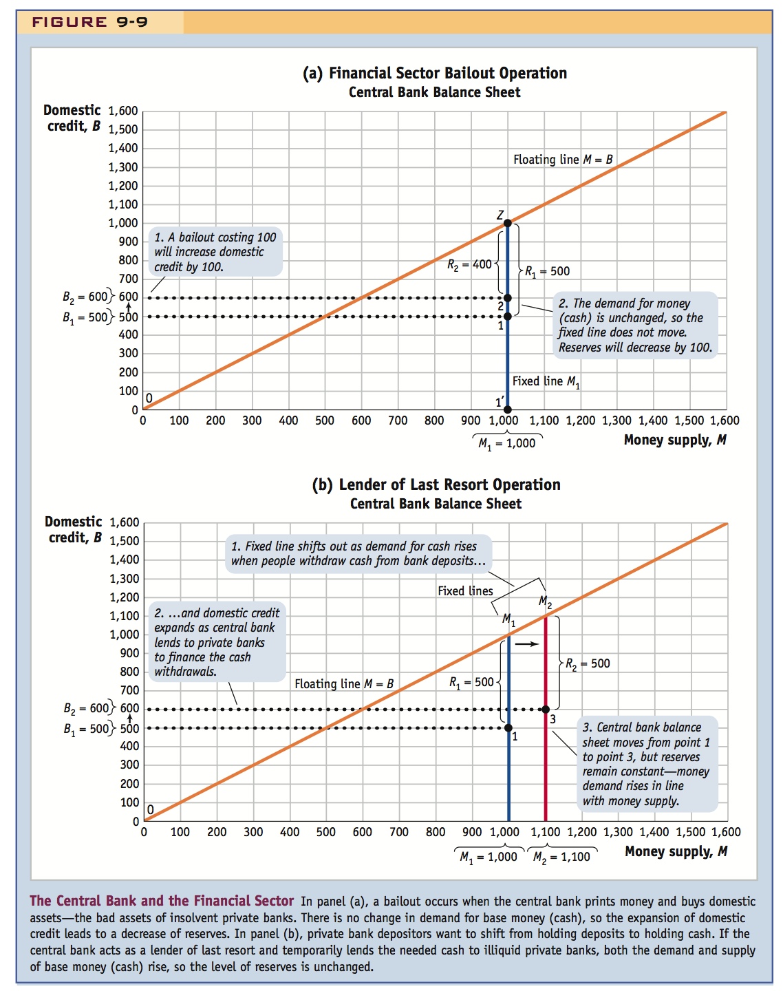
• Insolvency and bailouts. A private bank is insolvent if the value of its liabilities (e.g., customers’ deposits) exceeds the value of its assets (e.g., loans, other securities, and cash on hand). Often, this happens when the bank’s assets unexpectedly lose value (loans turn bad, stocks crash). In some circumstances, the government may offer a rescue or bailout to banks in such a damaged state, because it may be unwilling to see the bank fail (for political or even for economic reasons, if the bank provides valuable intermediation services to the economy). This bailout could be direct from the finance ministry. But the rescue may happen another way, and even in stages, if the banks ask for a loan from the central bank ostensibly for temporary liquidity purposes, and then (after losses appear) find their loans rolled over for a very long time, or even forgiven with some or all interest and principal unpaid.
  Suppose the central bank balance sheet was originally 500 reserves and 500 domestic credit, with base money supply of 1,000. The cash from a bailout (say, 100) goes to the private bank and domestic credit rises (by 100) to 600 on the central bank’s balance sheet. Because there has been no increase in base money demand, but more cash has gone into circulation, reserves must fall (by 100) to 400, as in Figure 9-9, panel (a). This central bank action is equivalent to the central bank buying bonds worth 100 directly from the government (a sterilization, as we saw previously) and the government then bailing out the private bank with the proceeds. Bottom line: bailouts are very risky for the central bank because they cause reserves to drain, endangering the peg.
• Illiquidity and bank runs. A private bank may be solvent, but it can still be illiquid: it holds some cash, but its loans cannot be sold (liquidated) quickly at a high price and depositors can withdraw at any time. If too many depositors attempt to withdraw their funds at once, the bank is in trouble if it has insufficient cash on hand: this is known as a bank run. In this situation, the central bank may lend money to commercial banks that are running out of cash. Suppose, for example, the monetary base is M0 and equals 1,000 as in the last example, but broad money is M2 (including bank deposits) and equals 2,000. The difference of 1,000 is the value of bank checking and saving deposits. If there is a run at a bank, and customers rush in and demand 100 in cash, the bank has to borrow 100 from somewhere to satisfy them. We suppose the bank is at zero cash or at the lowest level permitted by regulation—so it is constrained. Because every other bank is likewise constrained, fearful of lending to the troubled bank, or also experiencing a run, the problem cannot be solved by interbank lending. The central bank is then the lender of last resort. Crucially, in addition to the central bank expanding domestic credit (by 100) to 600, base money demand (demand for cash) also rises (by 100) to 1,100. Thus, we have a combination of the two types of shocks we have studied: an increase in domestic credit and an increase in (base) money demand, as shown in Figure 9-9, panel (b). Reserves do not change; they stay at 500. Why? The central bank is satisfying a demand for more cash, which absorbs the expansion of domestic credit. The situation will revert to normal when the run ends and the private bank pays back its loan to the central bank. Bottom line: providing liquidity to solvent banks is not risky for the central bank because there is no reserve drain to threaten the peg.

This simple classification of banks as insolvent or illiquid is useful but the reality is more complex. The difference between insolvency and illiquidity is often unclear. If depositors fear that banks have either problem, and that the central bank may bail them out slowly or partially, they will seek to withdraw their deposits and put them in a safe place. If the problems are potentially big, the fear may affect all depositors and all banks, and depositors will not be able to tell which banks are safe, which are illiquid, and which are insolvent. The problem gets more dangerous if the financial system is more complex, when banks have borrowing relationships with each other, for if one suffers losses and fails then it will cause spillover losses for others, and more possible failures. In many emerging markets and developing countries, this kind of panic often leads depositors to hold foreign bank deposits instead of deposits in local currency. This flight to foreign bank deposits happens because depositors do not know if, when, or how much of a bailout will occur. Thus they cannot be sure if the peg will hold, and if their peso deposits will in the end keep their value in dollar terms. In such circumstances, depositors’ fears can be self-fulfilling. A bank that faces a run may have to sell illiquid assets in a hurry at a low price, damaging itself and magnifying the problem. As depositors demand foreign currency, they drain reserves and make it more likely that devaluation will happen. A country at risk for devaluation faces a higher-risk premium, which in turn worsens economic conditions and encourages a flight from the domestic currency. If a depreciation happens, then banks and firms that have foreign currency liabilities will be in even worse shape, so running looks even better. And so the vicious circle continues.

The Old Lady doth protest too much: In September 2007, the Bank of England assured Northern Rock depositors that the bank would not fail. The bank’s balance sheet was widely believed to be healthy (solvency), but the bank had run short of cash to fund mortgages (illiquidity). Despite official assurances, there was a run on the bank because depositors preferred cash in hand to government promises.

Ben Stansall/AFP/Getty Images

To get a sense of the challenges faced by a central bank when confronted with difficulties in the banking sector under a fixed exchange rate, let us return to the case of Argentina after the Mexican Tequila crisis.

The Central Bank Balance Sheet and the Financial System

We can see from the experiences of Argentina and many other countries that the existence of a financial system affects the operations and balance sheet of the central bank. In particular, whether as a result of its own policy choices, formal laws and regulations, or political pressure, the typical central bank takes on the responsibility for monitoring, regulating, and—in an emergency—protecting a country’s commercial banking system.

A More General Balance Sheet As a result of its interactions with banks, the central bank’s balance sheet is in reality more complicated than we have assumed in our simplified model. Typically, it looks something like this, with some hypothetical values inserted:15

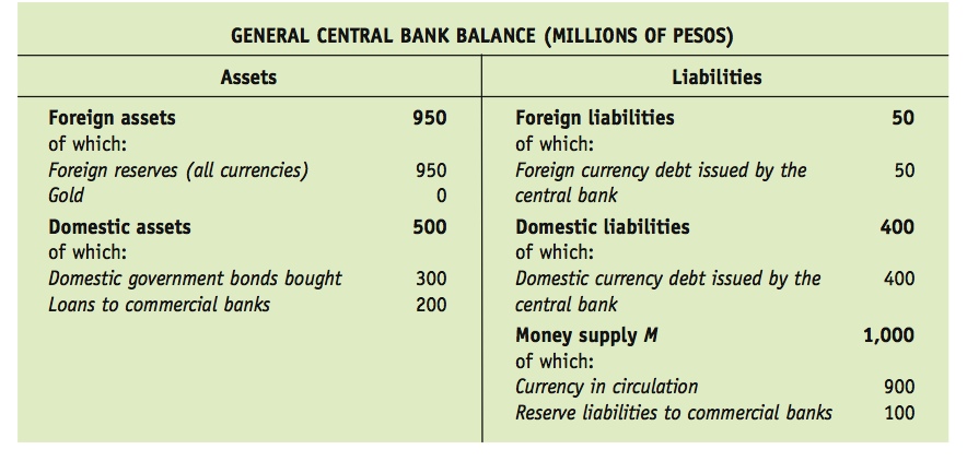
In the first row, the central bank’s net foreign assets are worth 900, given by 950 minus 50. We see that foreign assets can include other currencies besides the anchor currency (the dollar) and may also include gold. There may also be offsetting foreign liabilities if the central bank chooses to borrow. In this example, gold happens to be 0, foreign reserves are 950, and foreign liabilities are 50.

In the second row, net domestic assets are worth 100, 500 minus 400. We see that domestic assets may be broken down into government bonds (here, 300) and loans to commercial banks (here, 200). All of these assets can be offset by domestic liabilities, such as debt issued in home currency by the central bank. In this example, the central bank has issued 400 in domestic debt, which we shall assume was used to finance the purchase of foreign reserves.

Finally, the money supply is a liability for the central bank worth 1,000, as before. However, not all of that currency is “in circulation” (i.e., outside the central bank, in the hands of the public or in commercial bank vaults). Typically, central banks place reserve requirements on commercial banks and force them to place some cash on deposit at the central bank. This is considered a prudent regulatory device. In this case, currency in circulation is 900, and 100 is in the central bank as part of reserve requirements.

Despite all these refinements, the lessons of our simple model carry over. For example, in the simple approach, money supply (M) equaled foreign assets (R) plus domestic assets (B). We now see that, in general, money supply is equal to net foreign assets plus net domestic assets. The only real difference is the ability of the central bank to borrow by issuing nonmonetary liabilities, whether domestic or foreign.

Sterilization Bonds Why do central banks expand their balance sheets by issuing such liabilities? To see what the central bank can achieve by borrowing, consider what the preceding balance sheet would look like if the central bank had not borrowed to fund the purchase of reserves.

Without issuing domestic liabilities of 400 and foreign liabilities of 50, reserves would be lower by 450. In other words, they would fall from 950 to their original level of 500 seen in the example at the start of this chapter. Domestic credit would then be 500, as it was in that earlier example, with money supply of 1,000. Thus, what borrowing to buy reserves achieves is not a change in monetary policy (money supply and interest rates are unchanged, given the peg) but an increase in the backing ratio. Instead of a 50% backing ratio (500/1,000), the borrowing takes the central bank up to a 95% backing ratio (950/1,000).

But why stop there? What if the central bank borrowed, say, another 300 by issuing domestic debt and used the proceeds to purchase more reserves? Its domestic liabilities would rise from 400 to 700 (net domestic assets would fall from +100 to −200), and on the other side of the balance sheet, reserves (foreign assets) would rise from 950 to 1,250. Money supply would still be 1,000, but the backing ratio would be 125%. This could go on and on. Borrow another 250, and the backing ratio would be 150%.

As we have seen, these hypothetical operations are all examples of changes in the composition of the money supply—in terms of net foreign assets and net domestic assets—holding fixed the level of money supply. In other words, this is just a more general form of sterilization. And sterilization is just a way to change the backing ratio, all else equal.

What is new here is that the central bank’s net domestic assets (assets minus liabilities) can be less than zero because the central bank is now allowed to borrow. Many central banks do just this, by issuing bonds—or sterilization bonds as they are fittingly described. This allows the backing ratio to potentially exceed 100%.

Looking back at Figure 9-8, we could depict this by allowing reserves R to represent net foreign assets, credit B to represent net domestic assets, and B to be less than zero. The key equation M = R + B still holds, and the fixed and floating lines work as before, as long as we interpret zero net foreign assets as the trigger for a switch from fixed to floating.16 So we can imagine that the fixed line in Figure 9-8 can extend down below the horizontal axis.

Going below the horizontal axis means that net domestic credit is negative, and the backing ratio is more than 100%. Why might countries want backing to be that high? As we saw, Argentina had high backing of more than 70% on the eve of the Tequila crisis, but this would not have been enough for the peg to survive a major run from the financial system to dollars. In Figure 9-8, the zone below the horizontal axis would be an ultra-safe place, even farther from the floating line. Many countries have recently sought refuge in that direction (see Side Bar: The Great Reserve Accumulation in Emerging Markets).

The Great Reserve Accumulation in Emerging Markets

An illustration of reserve buildup via sterilization is provided by the activities of the People’s Bank of China, whose central bank balance sheet diagram is shown in Figure 9-10 in yuan (¥) units. The vertical distance to the 45-degree line represents net foreign assets R, which were essentially the same as foreign reserves because the bank had close to zero foreign liabilities.*

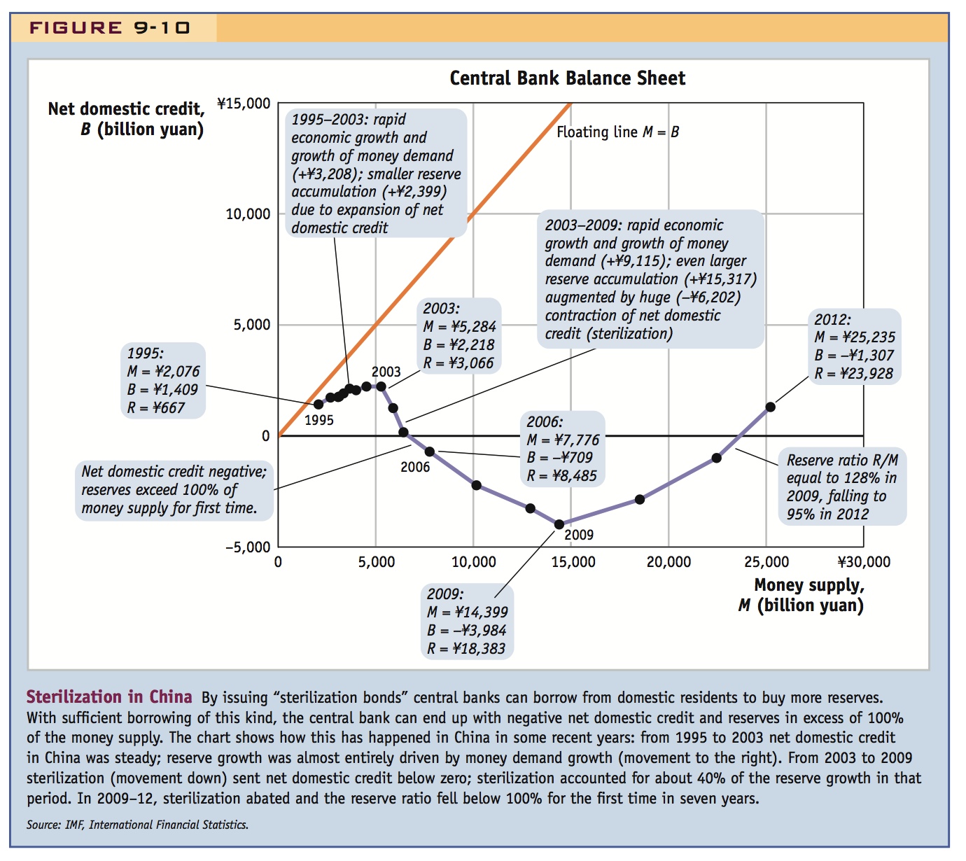
From 1995 to 2003 net domestic credit in China grew very slowly, from ¥1,409 billion to ¥2,218 billion, but rapid economic growth and financial development caused base money demand to grow rapidly, more than doubling, from ¥2,076 billion to ¥5,284 billion. Thus, most of the base money supply growth of ¥3,208 billion was absorbed by ¥2,399 billion of reserve accumulation. In this period, the backing ratio rose from 32% to 58%.

From 2003 to 2009 net domestic credit fell by ¥6,202 billion and eventually turned negative as the central bank sold large amounts of sterilization bonds. Money supply growth continued, rising from ¥5,284 billion to ¥14,399 billion, an increase of ¥9,115 billion. But the sterilization caused reserves to rise by almost twice as much, by ¥15,317 billion. The backing ratio rose from 58% to 128%. In the years 2009 to 2012 sterilization was not in play, and both reserves and domestic credit increased together; by 2012 money supply was ¥25,235 billion with 95% backing in reserves of ¥23,928.

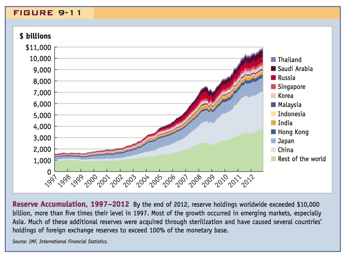
Given the country’s economic (and political) importance, the Chinese case attracts a lot of attention—but it isn’t the only example of this type of central bank behavior. Figure 9-11 shows the massive increase in reserves at central banks around the world in recent years: it started in about 1999, it mostly happened in Asia in countries pegging (more or less) to the dollar, and much of it was driven by large-scale sterilization. What was going on?

377

Causes of the Reserve Accumulation

Why are these countries, most of them poor emerging markets, accumulating massive hoards of reserves? There are various possible motivations for these reserve hoards, in addition to simply wanting greater backing ratios to absorb larger shocks to money demand.** For example, the countries may fear a sudden stop, when access to foreign capital markets dries up. Foreign creditors may cease to roll over short-term debt for a while, but if reserves are on hand, the central bank can temporarily cover the shortfall. This precautionary motive leads to policy guidelines or rules suggesting that an adequate and prudent level of reserves should be some multiple either of foreign trade or of short-term debt. In practice, such ratios usually imply reserve levels less than 100% of M0, the narrow money supply.

An alternative view, illustrated by the case of Argentina that we studied, would tend to focus on a different risk, the fragility of the financial sector. If there is a major banking crisis with a flight from local deposits to foreign banks, then a central bank may need a far greater level of reserves, adequate to cover some or all of M2, the broader measure of money that includes deposits and other liquid commercial bank liabilities. Because M2 can be several times M0, the reserve levels adequate for these purposes could be much larger and well over 100% of M0. Because reserves now far exceed traditional guidelines based on trade or debt levels, fears of financial fragility might be an important part of the explanation for the scale of the reserve buildup, with reserve backing in excess of 100% of M0. As economist Martin Feldstein pointed out after the Asian crisis, it is unrealistic to expect safe and crisis-free banking sector operations in emerging markets (in 2007 and 2008 we even saw bank runs in “developed countries” like the United Kingdom and the United States). But if countries are pegged, they then need to watch out for the peg:”…Sufficient liquidity, either through foreign currency reserves or access to foreign credit, would let a government restructure and recapitalize its banks without experiencing a currency crisis. The more international liquidity a government has, the less depositors will feel that they must rush to convert their currency before the reserves are depleted. And preventing a currency decline can be the best way to protect bank solvency.”^†

Thus, current reserve levels can be seen as a reaction, in part, to the financial crises of the recent past: policy makers have taken a “never again” stance, and have piled up a large war chest of reserves to guard against any risk of exchange rate crises. Is this wise? The benefits may seem clear, but many economists think this “insurance policy” carries too heavy an economic cost as countries invest in low-interest reserves and forsake investments with higher returns.

^* In this period, foreign liabilities were just 1% of foreign assets.

^** For a survey of the various possible explanations of the reserve buildup, see Joshua Aizenman, 2008, “Large Hoarding of International Reserves and the Emerging Global Economic Architecture,” Manchester School, 76(5): 487–503; Olivier Jeanne, 2007, “International Reserves in Emerging Market Countries: Too Much of a Good Thing?” Brookings Papers on Economic Activity, 38(1): 1–80.

^†See Martin S. Feldstein, March 1999, “A Self-Help Guide for Emerging Markets,” Foreign Affairs. 78(2), 93–109.

Summary

In this section, we examined the constraints on the operations of the central bank when a fixed exchange rate is in operation. We focused on the central bank balance sheet, which in its simplest form describes how the narrow money supply (monetary base) is backed by foreign assets (reserves) and domestic assets (domestic credit). We have seen how, in response to money demand shocks, the central bank buys or sells reserves, to defend the peg. The central bank can also change the composition of the money supply through sterilization operations, which keep the money supply constant.

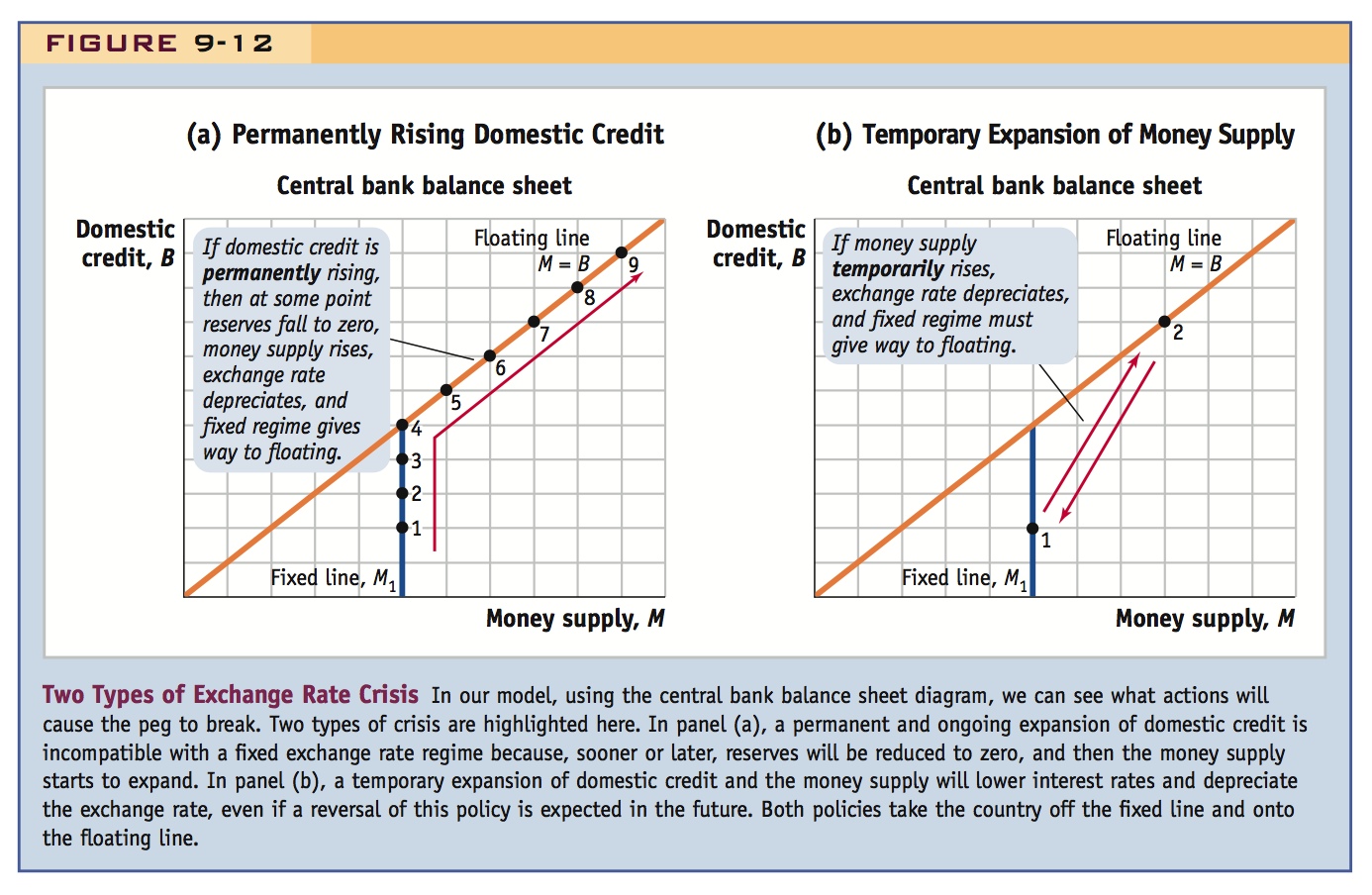
Two Types of Exchange Rate Crises When reserves go to zero, the country is floating, changes in domestic credit cause changes in the money supply, and the peg breaks. The central bank balance sheet diagrams in Figure 9-12 show two ways in which pegs can break:

• In panel (a), in the first type of crisis, domestic credit is constantly expanding, so the central bank is pushed up the fixed line until reserves run out. At this point, the currency floats, the money supply then grows without limit, and, in the long run, the exchange rate depreciates.
• In panel (b), in the second type of crisis, no long-run tendency exists for the money supply to grow, but there is a short-run temptation to expand the money supply temporarily, leading to a temporarily lower interest rate and a temporarily depreciated exchange rate.

In the next two sections, we develop models of these two types of crisis. Although the descriptions just given appear simple, a deeper examination reveals some peculiar features that illustrate the powerful role played by market expectations in triggering crises.