feenstrataylorintltrade3

2 Earnings of Labor

1. Objectives:
Since there are overall gains from trade, someone must benefit. But who loses? Analyze how trade affects factor returns.

2. Determination of Wages
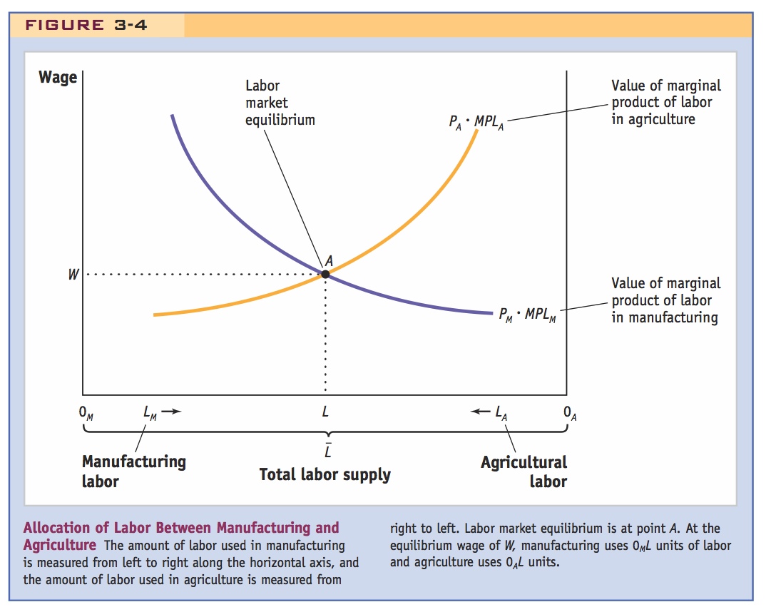
Derive Figure 3-4: Depict VMPL_M as a function of employment in manufacturing, L_M. Use the labor resource constraint to depict VMPL_A as a function of L_A.The equilibrium wage is determined where these intersect.

3. Change in the Relative Price of Manufactures
a. Effect on the Wage
We saw earlier that the relative price of the manufactured good P_M/P_A increases with trade. This can happen if either P_M increases or P_A decreases. Suppose the former: VMPL_M shifts up, so the wage increases and employment shifts into manufacturing.
b. Effect on Real Wages
Real wage in terms of food W/P_A has obviously increased? What about the real wage in terms of manufactured goods, W/P_M ? Geometrically, the increase in P_M causes VMPL_M to shift vertically more than W increases. So W/P_M must fall.
c. Overall Impact on Labor
Since W⁄P_A has increased and W/P_M has decreased trade has an ambiguous effect on the welfare of workers.
Notes: (1) Stark contrast with the Ricardian model, where the effect is unambiguous. (2) Serves as a salutary warning about making unqualified statements about the effects of trade on real wages.
d. Unemployment in the Specific-Factors Model
The model ignores unemployment. Two justifications: (1) Unemployment often considered a macroeconomic phenomenon. (2) Workers laid off in the contacting sector may find new jobs in the expanding sector. But the dislocations caused by such sectoral shifts are important.

Because there are overall gains from trade, someone in the economy must be better off, but not everyone is better off. The goal of this chapter is to explore how a change in relative prices, such as that shown in Figure 3-3, feeds back into the earnings of workers, landowners, and capital owners. We begin our study of the specific-factors model by looking at what happens to the wages earned by labor when there is an increase in the relative price of manufactures.

Determination of Wages

To determine wages, it is convenient to take the marginal product of labor in manufacturing (MPL_M), which was shown in Figure 3-1, panel (b), and the marginal product of labor in agriculture (MPL_A), and put them in one diagram.

First, we add the amount of labor used in manufacturing L_M and the amount used in agriculture L_A to give us the total amount of labor in the economy :

Figure 3-4 shows the total amount of labor on the horizontal axis. The amount of labor used in manufacturing L_M is measured from left (0_M) to right, while the amount of labor used in agriculture L_A is measured from right (0_A) to left. Each point on the horizontal axis indicates how much labor is used in manufacturing (measured from left to right) and how much labor is used in agriculture (measured from right to left). For example, point L indicates that 0_ML units of labor are used in manufacturing and 0_AL units of labor are used in agriculture, which adds up to units of labor in total.

Call this the value of marginal product of labor, as the graph does.

The second step in determining wages is to multiply the marginal product of labor in each sector by the price of the good in that sector (P_M or P_A). As we discussed earlier, in competitive markets, firms will hire labor up to the point at which the cost of one more hour of labor (the wage) equals the value of one more hour in production, which is the marginal product of labor times the price of the good. In each industry, then, labor will be hired until

W = P_M . MPL_M in manufacturing
W = P_A . MPL_M in agriculture

Students sometimes find this confusing at first. First, draw the VMPL in agriculture as a negative function of L_A. Then tell students to imagine picking up the graph and rotating it around.

In Figure 3-4, we draw the graph of P_M · MPL_M as downward-sloping. This curve is basically the same as the marginal product of labor MPL_M curve in Figure 3-1, panel (b), except that it is now multiplied by the price of the manufactured good. When we draw the graph of P_A · MPL_A for agriculture, however, it slopes upward. This is because we are measuring the labor used in agriculture L_A from right to left in the diagram: the marginal product of labor in agriculture falls as the amount of labor increases (moving from right to left).

Equilibrium Wage The equilibrium wage is found at point A, the intersection of the curves P_M · MPL_M and P_A · MPL_A in Figure 3-4. At this point, 0_ML units of labor are used in manufacturing, and firms in that industry are willing to pay the wage W = P_M · MPL_M. In addition, 0_AL units of labor are used in agriculture, and farmers are willing to pay the wage W = P_A · MPL_A. Because wages are equal in the two sectors, there is no reason for labor to move, and the labor market is in equilibrium.

Change in Relative Price of Manufactures

Now that we have shown how the wage is determined in the specific-factors model, we want to ask how the wage changes in response to an increase in the relative price of manufactures. That is, as the relative price of manufactures rises (shown in Figure 3-3), and the economy shifts from its no-trade equilibrium at point A to its trade equilibrium with production and consumption at points B and C, what is the effect on the earnings of each factor of production? In particular, what are the changes in the wage, and in the earnings of capital owners in manufacturing and landowners in agriculture?

Emphasize that this is a real model, so that it only determines real relative prices. Say that changing either P_A or P_M is just a graphical expedient to get at the effects of a change in the real relative price.

Effect on the Wage An increase in the relative price of manufacturing P_M/P_A can occur due to either an increase in P_M or a decrease in P_A. Both these price movements will have the same effect on the real wage; that is, on the amount of manufactures and food that a worker can afford to buy. For convenience, let us suppose that the price of manufacturing P_M rises, while the price of agriculture P_A does not change.

Invite them to reproduce the argument using P_A.

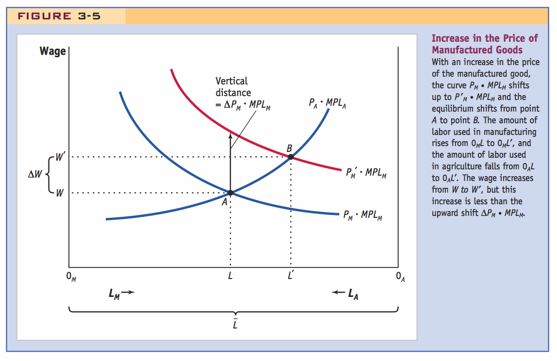
When P_M rises, the curve P_M · MPL_M shifts up to P′_M · MPL_M, as shown in Figure 3-5. The vertical rise in this curve is exactly ΔP_M · MPL_M, as illustrated in the diagram. (We use the symbol Δ, delta, to stand for the change in a variable.) The new intersection of the two curves occurs at point B, where the wage is W′ and the allocation of labor between the two sectors is identified by point L′. The equilibrium wage has risen from W to W′, the amount of labor used in the manufacturing sector has increased from 0_ML to 0_ML′, and the amount of labor used in agriculture has fallen from 0_AL to 0_AL′.

Effect on Real Wages The fact that the wage has risen does not really tell us whether workers are better off or worse off in terms of the amount of food and manufactured goods they can buy. To answer this question, we have to take into account any change in the prices of these goods. For instance, the amount of food that a worker can afford to buy with his or her hourly wage is W/P_A.5 Because W has increased from W to W′ and we have assumed that P_A has not changed, workers can afford to buy more food. In other words, the real wage has increased in terms of food.

Don't rush through this; some students might find it confusing.

The amount of the manufactured good that a worker can buy is measured by W/P_M. While W has increased, P_M has also increased, so at first glance we do not know whether W/P_M has increased or decreased. However, Figure 3-5 can help us figure this out. Notice that as we’ve drawn Figure 3-5, the increase in the wage from W to W′ is less than the vertical increase ΔP_M · MPL_M that occurred in the P_M · MPL_M curve. We can write this condition as

To see how W/P_M has changed, divide both sides of this equation by the initial wage W (which equals P_M · MPL_M) to obtain

where the final ratio is obtained because we canceled out MPL_M in the numerator and denominator of the middle ratio. The term ΔW/W in this equation is the percentage change in wages. For example, suppose the initial wage is $8 per hour and it rises to $10 per hour. Then ΔW/W = $2/$8 = 0.25, which is a 25% increase in the wage. Similarly, the term ΔP_M/P_M is the percentage change in the price of manufactured goods. When ΔW/W <; ΔP_M/P_M, then the percentage increase in the wage is less than the percentage increase in the price of the manufactured good. This inequality means that the amount of the manufactured good that can be purchased with the wage has fallen, so the real wage in terms of the manufactured good W/P_M has decreased.6

Overall Impact on Labor We have now determined that as a result of our assumption of an increase in the relative price of manufactured goods, the real wage in terms of food has increased and the real wage in terms of the manufactured good has decreased. In this case, we assumed that the increase in relative price was caused by an increase in the price of manufactures with a constant price of agriculture. Notice, though, that if we had assumed a constant price of manufactures and a decrease in the price of agriculture (taken together, an increase in the relative price of manufactures), then we would have arrived at the same effects on the real wage in terms of both products.

Emphasize this punchline . . .

Is labor better off or worse off after the price increase? We cannot tell. People who spend most of their income on manufactured goods are worse off because they can buy fewer manufactured goods, but those who spend most of their income on food are better off because more food is affordable. The bottom line is that in the specific-factors model, the increase in the price of the manufactured good has an ambiguous effect on the real wage and therefore an ambiguous effect on the well-being of workers.

. . .and its real world implications.

The conclusion that we cannot tell whether workers are better off or worse off from the opening of trade in the specific-factors model might seem wishy-washy to you, but it is important for several reasons. First, this result is different from what we found in the Ricardian model of Chapter 2, in which the real wage increases with the opening of trade so that workers are always unambiguously better off than they are in the absence of trade.7 In the specific-factors model, that is no longer the case; the opening of trade and the shift in relative prices raise the real wage in terms of one good but lower it in terms of the other good. Second, our results for the specific-factors model serve as a warning against making unqualified statements about the effect of trade on workers, such as “Trade is bad for workers” or “Trade is good for workers.” Even in the specific-factors model, which is simplified by considering only two industries and not allowing capital or land to move between them, we have found that the effects of opening trade on the real wage are complicated. In reality, the effect of trade on real wages is more complex still.

Return to the theme of the "realism" of the assumption that labor is perfectly mobile: it is a useful first approximation for the problem at hand.

Unemployment in the Specific-Factors Model We have ignored one significant, realistic feature in the specific-factors model: unemployment. You may often see news stories about workers who are laid off because of import competition and who face a period of unemployment. Despite this outcome, most economists do not believe that trade necessarily harms workers overall. It is true that we have ignored unemployment in the specific-factors model: the labor employed in manufacturing L_M plus the labor employed in agriculture L_A always sums to the total labor supply , which means that there is no unemployment. One of the reasons we ignore unemployment in this model is that it is usually treated as a macroeconomic phenomenon, caused by business cycles, and it is hard to combine business cycle models with international trade models to isolate the effects of trade on workers. But the other, simpler reason is that even when people are laid off because of import competition, many of them find new jobs within a reasonable period, and sometimes they find jobs with higher wages, as shown in the next application. Therefore, even if we take into account spells of unemployment, once we recognize that workers can find new jobs—possibly in export industries that are expanding—then we still cannot conclude that trade is necessarily good or bad for workers.

This may require some review of different sorts of unemployment, with some elaboration on "cyclical" unemployment.

In the two applications that follow, we look at some evidence from the United States on the amount of time it takes to find new jobs and on the wages earned, and at attempts by governments to compensate workers who lose their jobs because of import competition. This type of compensation is called Trade Adjustment Assistance (TAA) in the United States.

Comparison of employment, wages, and layoffs in manufacturing and services. Lessons: (1) Wages do not equalize across sectors. (2) Layoffs are common, but may be caused by other things than import competition. (3) (More than half but not all) displaced workers usually find new jobs within two or three years, but at lower wages. (4) Real wages for production workers fell from 1979 to 1995. They have increased slightly since then, while real wages in the service sectors have increased more.

Manufacturing and Services in the United States: Employment and Wages Across Sectors

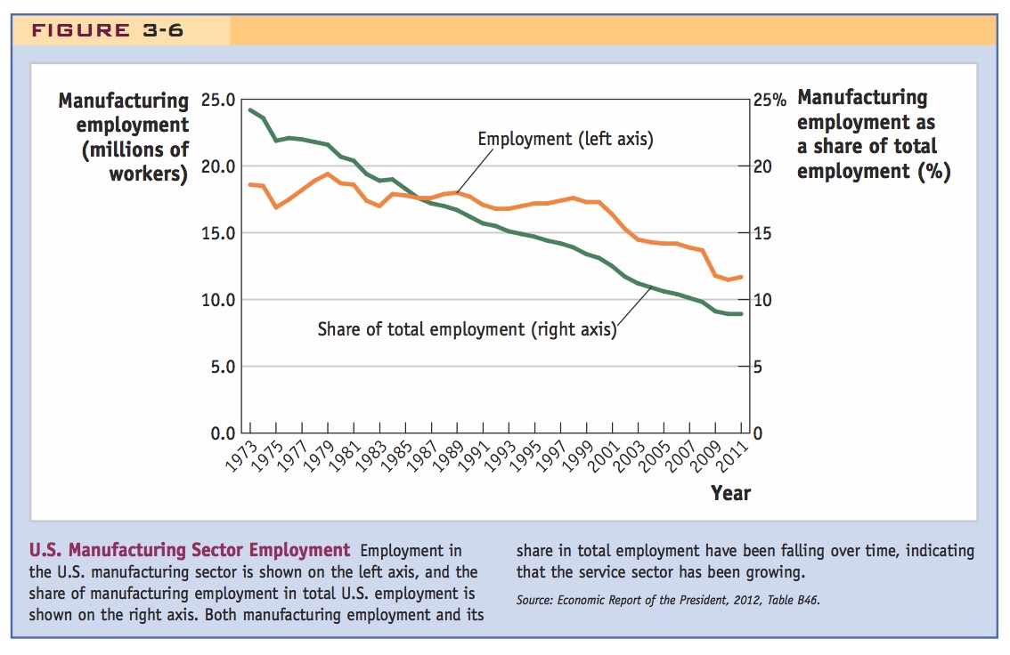
Although the specific-factors model emphasizes manufacturing and agriculture, the amount of labor devoted to agriculture in most industrialized countries is small. A larger sector in industrialized countries is that of services, which includes wholesale and retail trade, finance, law, education, information technology, software engineering, consulting, and medical and government services. In the United States and most industrial countries, the service sector is larger than the manufacturing sector and much larger than the agriculture sector.

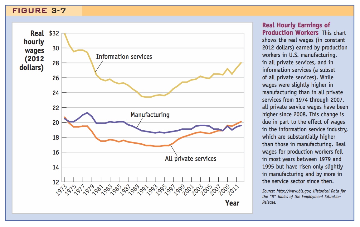
In Figure 3-6, we show employment in the manufacturing sector of the United States, both in terms of the number of workers employed in it and as a percentage of total employment in the economy. Using either measure, employment in manufacturing has been falling over time; given zero or negative growth in the agriculture sector, this indicates that the service sector has been growing. In Figure 3-7, we show the real wages earned by production—or blue-collar—workers in manufacturing, in all private services, and in information services (a subset of private services).8 While wages were slightly higher in manufacturing than in private services from 1974 through 2007, all private service wages have been higher since 2008. This change is due in part to the effect of wages in the information service industry, which are substantially higher than those in manufacturing. For example, average hourly earnings in all private services were $19.90 per hour in 2012 and slightly lower—$19.60 per hour—in manufacturing overall. But in information services, average wages were much higher—$28.00 per hour.

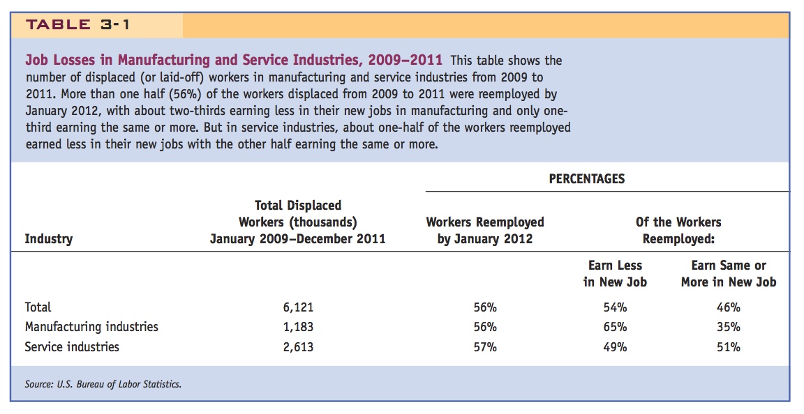
In both manufacturing and services, many workers are displaced or laid off each year and need to look for other jobs. In the three years from January 2009 to December 2011, for example, about 1.2 million workers were displaced in manufacturing and 2.6 million in all service industries, as shown in Table 3-1. Of those laid off in manufacturing, 56% were reemployed by January 2012, and about two-thirds of these (65%) earned less in their new jobs and only one-third earned the same or more. For services, while a similar fraction 57% were reemployed by January 2012, slightly more than one-half of these (51%) earned the same or more in their new jobs. So the earnings of those displaced in the service sectors do not suffer as much as the earnings of workers displaced from manufacturing.

There are four lessons that we can take away from this comparison of employment and wages in manufacturing and services. First, wages differ across different sectors in the economy, so our theoretical assumption that wages are the same in agriculture and manufacturing is a simplification. Second, many workers are displaced each year and must find jobs elsewhere. Some of these workers may be laid off due to competition from imports, but there are other reasons, too—for instance, products that used to be purchased go out of fashion, firms reorganize as computers and other technological advances become available, and firms change locations. Third, more than one-half of displaced workers find a new job within two or three years but not necessarily at the same wage. Typically, older workers (age 45 to 64) experience earnings losses when shifting between jobs, whereas younger workers (age 25 to 44) are often able to find a new job with the same or higher wages. Finally, when we measure wages in real terms by adjusting for inflation in the price of consumer goods, we see that real wages for all production workers fell in most years between 1979 and 1995 (we examine the reasons for that fall in later chapters). The real wages for production workers in manufacturing have risen only slightly since then, while the real wages for service workers have risen by more, so that workers in services now have higher earnings than those in manufacturing on average (and especially so for workers in information services).

These are important facts with which students should be familiar.

Trade Adjustment Assistance (TAA) programs offer insurance and health benefits to workers laid off because of import competition. Economists recommended a similar program to mitigate the dislocation in East Germany when it reunited with West Germany.

Trade Adjustment Assistance Programs: Financing the Adjustment Costs of Trade

Should the government step in to compensate workers who are looking for jobs or who do not find them in a reasonable period? The unemployment insurance program in the United States provides some compensation, regardless of the reason for the layoff. In addition, the Trade Adjustment Assistance (TAA) program offers additional unemployment insurance payments and health insurance to workers who are laid off because of import competition and who are enrolled in a retraining program. The quotation from President Kennedy at the beginning of the chapter comes from a speech he made introducing the TAA program in 1962. He believed that this program was needed to compensate those Americans who lost their jobs due to international trade. Since 1993 there has also been a special TAA program under the North American Free Trade Agreement (NAFTA) for workers who are laid off as a result of import competition from Mexico or Canada.9 Recently, as part of the jobs stimulus bill signed by President Obama on February 17, 2009, workers in the service sector (as well as farmers) who lose their jobs due to trade can now also apply for TAA benefits. This extension is described in Headlines: Services Workers Are Now Eligible for Trade Adjustment Assistance.

Other countries also have programs like TAA to compensate those harmed by trade. A particularly interesting example occurred with the unification of East and West Germany on June 30, 1990. On that date, all barriers to trade between the countries were removed as well as all barriers to the movement of labor and capital between the two regions. The pressure from labor unions to achieve wage parity (equality) between the East and West meant that companies in former East Germany were faced with wages that were far above what they could afford to pay. According to one estimate, only 8% of former East German companies would be profitable at the higher wages paid in the West. In the absence of government intervention, it could be expected that severe bankruptcy and unemployment would result, leading to massive migration of East German workers to the former West Germany.

Economists studying this situation proposed that deep wage subsidies, or “flexible employment bonuses,” should be given in former East Germany, thereby allowing factories to employ their workers while paying only a fraction of their wages. Furthermore, they argued that the wage subsidies would essentially pay for themselves because without them the government would have to provide unemployment insurance on a massive scale to the people left without jobs.10 As it turns out, wage subsidies of this type were not used, and unemployment in the East and migration to the West continue to be challenging policy issues for the united Germany. According to the 2011 census and recent studies, the East–West differences still remain with the East having higher unemployment and lower wages than found in the West of Germany.11