feenstrataylorintltrade3

1 Heckscher-Ohlin Model

1. Objective: Develop the model and explain how factor endowments affect trade
2x2x2 model: Two countries, Home and Foreign; two goods, computers and shoes; two factors, labor and capital, both supplied inelastically

2. Assumptions of the Heckscher-Ohlin Model
Assumption 1: Both factors can move freely between the industries.
This is unlike specific-factors, where one factor is stuck in each sector.
Assumption 2: Shoe production is labor-intensive: it takes more labor per unit capital to produce shoes than computers. Conversely, computers are capital-intensive.
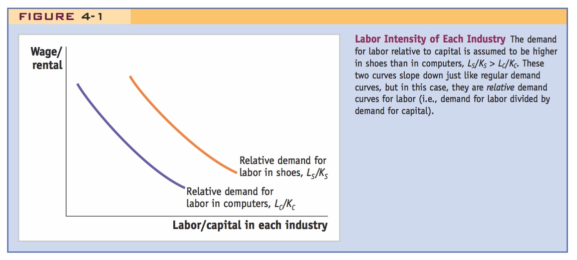
Plot relative demand curves for labor (demand for labor/demand for capital) against the wage/rental ratio, W/R. The relative demand for labor is shoes is higher because shoes are labor-intensive.
Assumption 3: Foreign is labor-abundant, so the labor–capital ratio is higher abroad than at Home. Conversely, Home is capital-abundant.
Note that factor endowments may change (immigration, investment), but that we take them as exogenous for the purposes of this model.
Assumption 4: Goods can be traded freely across countries, but factors do not move between countries.
Chapter 5 will allow factor mobility.
Assumption 5: Technologies are identical in the two countries.
Not a realistic assumption, but designed to focus on the effects of factor endowments on trade.
Assumption 6: Preferences are identical in both countries, and do not vary with income.
Just a simplifying assumption: It means that a poor country will demand the same ratio of shoes to computers as a rich country will.

In building the Heckscher-Ohlin model, we suppose there are two countries, Home and Foreign, each of which produces two goods, computers and shoes, using two factors of production, labor and capital. Using symbols for capital (K) and labor (L), we can add up the resources used in each industry to get the total for the economy. For example, the amount of capital Home uses in shoes K_S, plus the amount of capital used in computers K_C, adds up to the total capital available in the economy , so that K_C + K_S = . The same applies for Foreign: . Similarly, the amount of labor Home uses in shoes L_S, and the amount of labor used in computers L_C, add up to the total labor in the economy , so that L_C + L_S = . The same applies for Foreign: .

Assumptions of the Heckscher-Ohlin Model

Because the Heckscher-Ohlin (HO) model describes the economy in the long run, its assumptions differ from those in the short-run specific-factors model of Chapter 3:

Say that this is what makes a long-run model.

Assumption 1: Both factors can move freely between the industries.

This assumption implies that if both industries are actually producing, then capital must earn the same rental R in each of them. The reason for this result is that if capital earned a higher rental in one industry than the other, then all capital would move to the industry with the higher rental and the other industry would shut down. This result differs from the specific-factors model in which capital in manufacturing and land in agriculture earned different rentals in their respective industries. But like the specific-factor model, if both industries are producing, then all labor earns the same wage W in each of them.

Our second assumption concerns how the factors are combined to make shoes and computers:

Assumption 2: Shoe production is labor-intensive; that is, it requires more labor per unit of capital to produce shoes than computers, so that L_S/K_S > L_C/K_C.

Another way to state this assumption is to say that computer production is capital-intensive; that is, more capital per worker is used to produce computers than to produce shoes, so that K_C/L_C > K_S/L_S. The idea that shoes use more labor per unit of capital, and computers use more capital per worker, matches how most of us think about the technologies used in these two industries.

This is confusing to students at first, since it is the demand for the RATIO of L to K, as a function of the RATIO of factor prices W/R.

In Figure 4-1, the demands for labor relative to capital in each industry (L_C/K_C and L_S/K_S) are graphed against the wage relative to the rental on capital, W/R (or the wage-rental ratio). These two curves slope down just like regular demand curves: as W/R rises, the quantity of labor demanded relative to the quantity of capital demanded falls. As we work through the HO model, remember that these are relative demand curves for labor; the “quantity” on the horizontal axis is the ratio of labor to capital used in production, and the “price” is the ratio of the labor wage to the capital rental. Assumption 2 says that the relative demand curve in shoes, L_S/K_S in Figure 4-1, lies to the right of the relative demand curve in computers L_C/K_C, because shoe production is more labor-intensive.

Whereas the preceding assumptions have focused on the production process within each country, the HO model requires assumptions that apply across countries as well. Our next assumption is that the amounts of labor and capital found in Home and Foreign are different:

Assumption 3: Foreign is labor-abundant, by which we mean that the labor–capital ratio in Foreign exceeds that in Home, . Equivalently, Home is capital-abundant, so that .

There are many reasons for labor, capital, and other resources to differ across countries: countries differ in their geographic size and populations, previous waves of immigration or emigration may have changed a country’s population, countries are at different stages of development and so have differing amounts of capital, and so on. If we are considering land in the HO model, Home and Foreign will have different amounts of usable land due to the shape of their borders and to differences in topography and climate. In building the HO model, we do not consider why the amounts of labor, capital, or land differ across countries but simply accept these differences as important determinants of why countries engage in international trade.

Assumption 3 focuses on a particular case, in which Foreign is labor-abundant and Home is capital-abundant. This assumption is true, for example, if Foreign has a larger workforce than Home () and Foreign and Home have equal amounts of capital, . Under these circumstances, , so Foreign is labor-abundant. Conversely, the capital–labor ratio in Home exceeds that in Foreign, , so the Home country is capital-abundant.

Assumption 4: The final outputs, shoes and computers, can be traded freely (i.e., without any restrictions) between nations, but labor and capital do not move between countries.

In this chapter, we do not allow labor or capital to move between countries. We relax this assumption in the next chapter, in which we investigate the movement of labor between countries through immigration as well as the movement of capital between countries through foreign direct investment.

Our final two assumptions involve the technologies of firms and tastes of consumers across countries:

Suggestion for more advanced students: Specify that we are assuming constant returns to scale. This justifies the dependence of MPs on L/K, as well the assumption later that an increase in L raises MPK (and vice versa).

Assumption 5: The technologies used to produce the two goods are identical across the countries.

This assumption is the opposite of that made in the Ricardian model (Chapter 2), which assumes that technological differences across countries are the reason for trade. It is not realistic to assume that technologies are the same across countries because often the technologies used in rich versus poor countries are quite different (as described in the following application). Although assumption 5 is not very realistic, it allows us to focus on a single reason for trade: the different amounts of labor and capital found in each country. Later in this chapter, we use data to test the validity of the HO model and find that the model performs better when assumption 5 is not used.

Our final assumption is as follows:

Assumption 6: Consumer tastes are the same across countries, and preferences for computers and shoes do not vary with a country’s level of income.

That is, we suppose that a poorer country will buy fewer shoes and computers, but will buy them in the same ratio as a wealthier country facing the same prices. Again, this assumption is not very realistic: consumers in poor countries do spend more of their income on shoes, clothing, and other basic goods than on computers, whereas in rich countries a higher share of income can be spent on computers and other electronic goods than on footwear and clothing. Assumption 6 is another simplifying assumption that again allows us to focus attention on the differences in resources as the sole reason for trade.

No, it is possible for an industry to be labor-intensive in one country, but capital-intensive in another. Examples: Shoe plants in Asia (labor-intensive) and in Maine (capital-intensive). Ignore such factor intensity reversals to get clean results about factor returns.

Are Factor Intensities the Same Across Countries?

One of our assumptions for the Heckscher-Ohlin (HO) model is that the same good (shoes) is labor-intensive in both countries. Specifically, we assume that in both countries, shoe production has a higher labor–capital ratio than does computer production. Although it might seem obvious that this assumption holds for shoes and computers, it is not so obvious when comparing other products, say, shoes and call centers.

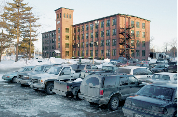
Despite its nineteenth-century exterior, this New Balance factory in Maine houses advanced shoe-manufacturing technology.

AP Photo/Robert F. Bukaty

In principle, all countries have access to the same technologies for making footwear. In practice, however, the machines used in the United States are different from those used in Asia and elsewhere. While much of the footwear in the world is produced in developing nations, the United States retains a small number of shoe factories. New Balance, which manufactures sneakers, has five plants in the New England states, and 25% of the shoes it sells in North America are produced in the United States. One of their plants is in Norridgewock, Maine, where employees operate computerized equipment that allows one person to do the work of six.1 This is a far cry from the plants in Asia that produce shoes for Nike, Reebok, and other U.S. producers. Because Asian plants use older technology (such as individual sewing machines), they use more workers to operate less productive machines.

In call centers, on the other hand, technologies (and, therefore, factor intensities) are similar across countries. Each employee works with a telephone and a personal computer, so call centers in the United States and India are similar in terms of the amount of capital per worker that they require. The telephone and personal computer, costing several thousand dollars, are much less expensive than the automated manufacturing machines in the New Balance plant in the United States, which cost tens or hundreds of thousands of dollars. So the manufacture of footwear in the New Balance plant is capital-intensive as compared with a U.S. call center. In India, by contrast, the sewing machine used to produce footwear is cheaper than the computer used in the call center. So footwear production in India is labor-intensive as compared with the call center, which is the opposite of what holds in the United States. This example illustrates a reversal of factor intensities between the two countries.

The same reversal of factor intensities is seen when we compare the agricultural sector across countries. In the United States, agriculture is capital-intensive. Each farmer works with tens of thousands of dollars in mechanized, computerized equipment, allowing a farm to be maintained by only a handful of workers. In many developing countries, however, agriculture is labor-intensive. Farms are worked by many laborers with little or no mechanized equipment. The reason that this labor-intensive technology is used in agriculture in developing nations is that capital equipment is expensive relative to the wages earned.

In assumption 2 and Figure 4-1, we assume that the labor–capital ratio (L/K) of one industry exceeds that of the other industry regardless of the wage-rental ratio (W/R). That is, whether labor is cheap (as in a developing country) or expensive (as in the United States), we are assuming that the same industry (shoes, in our example) is labor-intensive in both countries. This assumption may not be true for footwear or for agriculture, as we have just seen. In our treatment of the HO model, we ignore the possibility of factor intensity reversals. The reason for ignoring these is to get a definite prediction from the model about the pattern of trade between countries so that we can see what happens to the price of goods and the earnings of factors when countries trade with one another.

No-Trade Equilibrium

3. No-Trade Equilibrium
a. Production Possibilities Frontiers
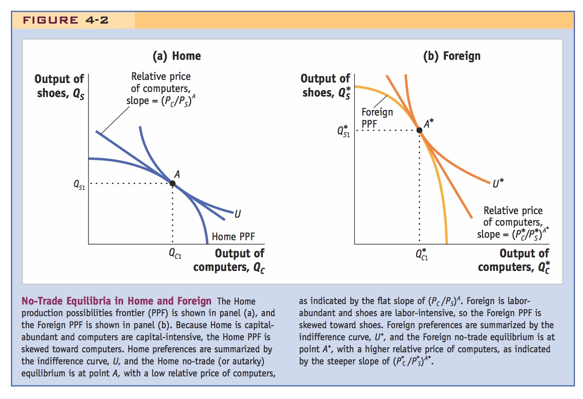
Since Home is capital-abundant and computers are capital-intensive, its PPF is skewed towards computers. Conversely, the Foreign PPF is skewed towards shoes.
b. Indifference Curves
Autarky equilibrium occurs where the indifference curve is tangent to the PPF. The slope of the common tangent line is the relative price of computers.
c. No-Trade Equilibrium Price
The relative price of computers will be low at Home, and high abroad. Intuition: Home is abundant in capital, so it produces a lot of the capital-intensive good.

In assumption 3, we outlined the difference in the amount of labor and capital found at Home and in Foreign. Our goal is to use these differences in resources to predict the pattern of trade. To do this, we begin by studying the equilibrium in each country in the absence of trade.

This follows from the Rybczynski theorem, developed in Chapter 5, but is intuitively clear enough just to assert here.

Production Possibilities Frontiers To determine the no-trade equilibria in Home and Foreign, we start by drawing the production possibilities frontiers (PPFs) in each country as shown in Figure 4-2. Under our assumptions that Home is capital-abundant and that computer production is capital-intensive, Home is capable of producing more computers than shoes. The Home PPF drawn in panel (a) is skewed in the direction of computers to reflect Home’s greater capability to produce computers. Similarly, because Foreign is labor-abundant and shoe production is labor-intensive, the Foreign PPF shown in panel (b) is skewed in the direction of shoes, reflecting Foreign’s greater capability to produce shoes. These particular shapes for the PPFs are reasonable given the assumptions we have made. When we continue our study of the Heckscher-Ohlin (HO) model in Chapter 5, we prove that the PPFs must take this shape.2 For now, we accept these shapes of the PPF and use them as the starting point for our study of the HO model.

Same caveat about community indifference curves as in Chapter 3.

Indifference Curves Another assumption of the HO model (assumption 6) is that consumer tastes are the same across countries. As we did in the Ricardian model, we graph consumer tastes using indifference curves. Two of these curves are shown in Figure 4-2 (U and U* for Home and Foreign, respectively); one is tangent to Home’s PPF, and the other is tangent to Foreign’s PPF. Notice that these indifference curves are the same shape in both countries, as required by assumption 6. They are tangent to the PPFs at different points because of the distinct shapes of the PPFs just described.

The slope of an indifference curve equals the amount that consumers are willing to pay for computers measured in terms of shoes rather than dollars. The slope of the PPF equals the opportunity cost of producing one more computer in terms of shoes given up. When the slope of an indifference curve equals the slope of a PPF, the relative price that consumers are willing to pay for computers equals the opportunity cost of producing them, so this point is the no-trade equilibrium.3 The common slope of the indifference curve and PPF at their tangency equals the relative price of computers P_C/P_S. A steeply sloped price line implies a high relative price of computers, whereas a flat price line implies a low relative price for computers.

No-Trade Equilibrium Price Given the differently shaped PPFs, the indifference curves of each country will be tangent to the PPFs at different production points, corresponding to different relative price lines across the two countries. In Home, the no-trade or autarky equilibrium is shown by point A, at which Home produces Q_C₁ of computers and Q_S₁ of shoes at the relative price of (P_C/P_S)^A. Because the Home PPF is skewed toward computers, the slope of the Home price line (P_C/P_S)^A is quite flat, indicating a low relative price of computers. In Foreign, the no-trade or autarky equilibrium is shown by point A* at which Foreign produces of computers and of shoes at the relative price of . Because the Foreign PPF is skewed toward shoes, the slope of the Foreign price line is quite steep, indicating a high relative price of computers. Therefore, the result from comparing the no-trade equilibria in Figure 4-2 is that the no-trade relative price of computers at Home is lower than in Foreign. (Equivalently, we can say that the no-trade relative price of shoes at Home is higher than in Foreign.)

Emphasize, as before, that differences in autarky prices drive trade. But now these differences are caused (via Rybczynski) by differences in factor endowments, rather than technologies.

These comparisons of the no-trade prices reflect the differing amounts of labor found in the two countries: the Foreign country has abundant labor, and shoe production is labor-intensive, so the no-trade relative price of shoes is lower in Foreign than in Home. That Foreigners are willing to give up more shoes for one computer reflects the fact that Foreign resources are suited to making more shoes. The same logic applies to Home, which is relatively abundant in capital. Because computer production is capital-intensive, Home has a lower no-trade relative price of computers than Foreign. Thus, Home residents need to give up fewer shoes to obtain one computer, reflecting the fact that their resources are suited to making more computers.

Free-Trade Equilibrium

4. Free-Trade Equilibrium
Derive the export supply and import demands for computers, then determine the world relative price of computers.
a. Home Equilibrium with Free Trade
Trade raises the relative price of computers relative to Home’s autarky price. Therefore, Home moves along its PPF, specializing more in computers and producing less shoes, and consuming on a higher indifference curve outside of its PPF. (Show the trade triangle.) It exports computers. The higher the relative price of computers, the more it exports: The export supply curve of computers is positively sloped.
b. Foreign Equilibrium with Free Trade
Trade lowers the relative price of computers relative to Foreign autarky price. Foreign specializes more in shoes and producing fewer computers. (Show the trade triangle.) It imports computers. The higher the relative price of computers, the less it imports: The import demand curve for computers is negatively sloped.
c. Equilibrium Price with Free Trade
Equilibrium occurs where export supply equals import demand. Note that trade triangles are of the same size.
d. Pattern of Trade
Home exports computers, while Foreign exports shoes. Therefore the result is: Heckscher-Ohlin theorem. With two goods and two factors, each country will export the good that uses intensively the factor of production it has in abundance and will import the other good.
Review how the six assumptions lead to this conclusion.

We are now in a position to determine the pattern of trade between the countries. To do so, we proceed in several steps. First, we consider what happens when the world relative price of computers is above the no-trade relative price of computers at Home, and trace out the Home export supply of computers. Second, we consider what happens when the world relative price is below the no-trade relative price of computers in Foreign, and trace out the Foreign import demand for computers. Finally, we put together the Home export supply and Foreign import demand to determine the equilibrium relative price of computers with international trade.

Home Equilibrium with Free Trade The first step is displayed in Figure 4-3. We have already seen in Figure 4-2 that the no-trade relative price of computers is lower in Home than in Foreign. Under free trade, we expect the equilibrium relative price of computers to lie between the no-trade relative prices in each country (as we already found in the Ricardian model of Chapter 2). Because the no-trade relative price of computers is lower at Home, the free-trade equilibrium price will be above the no-trade price at Home. Therefore, panel (a) of Figure 4-3 shows the Home PPF with a free-trade or world relative price of computers, (P_C/P_S)^W, higher than the no-trade Home relative price, (P_C/P_S)^A, shown in panel (a) of Figure 4-2.

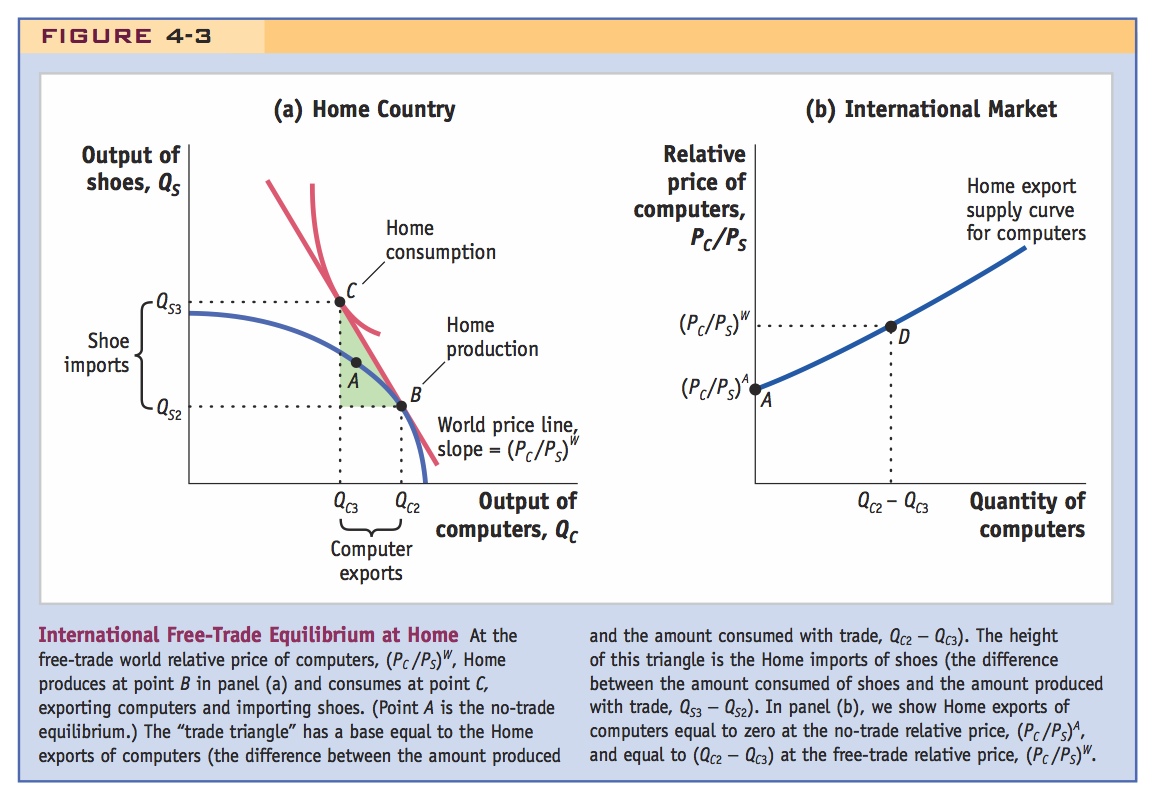
The no-trade equilibrium at Home, point A, has the quantities (Q_C₁, Q_S₁) for computers and shoes, shown in Figure 4-2. At the higher world relative price of computers, Home production moves from point A, (Q_C₁, Q_S₁), to point B in Figure 4-3, (Q_C₂, Q_S₂), with more computers and fewer shoes. Thus, with free trade, Home produces fewer shoes and specializes further in computers to take advantage of higher world relative prices of computers. Because Home can now engage in trade at the world relative price, Home’s consumption can now lie on any point along the world price line through B with slope (P_C/P_S)^W. The highest Home utility is obtained at point C, which is tangent to the world price line (P_C/P_S)^W and has the quantities consumed (Q_C₃, Q_S₃).

We can now define the Home “trade triangle,” which is the triangle connecting points B and C, shown in panel (a) of Figure 4-3. Point B is where Home is producing and point C is where it is consuming, and the line connecting the two points represents the amount of trade at the world relative price. The base of this triangle is the Home exports of computers (the difference between the amount produced and the amount consumed with trade, or Q_C₂ − Q_C₃). The height of this triangle is the Home imports of shoes (the difference between the amount consumed of shoes and the amount produced with trade, or Q_S₃ − Q_S₂).

In panel (b) of Figure 4-3, we graph the Home exports of computers against their relative price. In the no-trade equilibrium, the Home relative price of computers was (P_C/P_S)^A, and exports of computers were zero. This no-trade equilibrium is shown by point A in panel (b). Under free trade, the relative price of computers is (P_C/P_S)^W, and exports of computers are the difference between the amount produced and amount consumed with trade, or (Q_C₂ − Q_C₃). This free-trade equilibrium is shown by point D in panel (b). Joining up points A and D, we obtain the Home export supply curve of computers. It is upward-sloping because at higher relative prices as compared with the no-trade price, Home is willing to specialize further in computers to export more of them.

Foreign Equilibrium with Free Trade We proceed in a similar fashion for the Foreign country. In panel (a) of Figure 4-4, the Foreign no-trade equilibrium is at point A*, with the high equilibrium relative price of computers . Because the Foreign no-trade relative price was higher than at Home, and we expect the free-trade relative price to lie between, it follows that the free-trade or world equilibrium price of computers (P_C/P_S)^W is lower than the no-trade Foreign price .

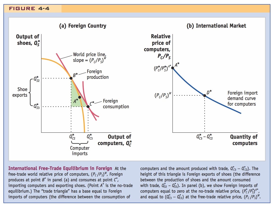
At the world relative price, Foreign production moves from point A*, (), to point B*, (), with more shoes and fewer computers. Thus, with free trade, Foreign specializes further in shoes and produces fewer computers. Because Foreign can now engage in trade at the world relative price, Foreign’s consumption can now lie on any point along the world price line through B* with slope (P_C/P_S)^W. The highest Foreign utility is obtained at point C*, which is tangent to the world price line (P_C/P_S)^W and has the quantities consumed (). Once again, we can connect points B* and C* to form a “trade triangle.” The base of this triangle is Foreign imports of computers (the difference between consumption of computers and production with trade, or ), and the height is Foreign exports of shoes (the difference between production and consumption with trade, or ).

In panel (b) of Figure 4-4, we graph Foreign’s imports of computers against its relative price. In the no-trade equilibrium, the Foreign relative price of computers was , and imports of computers were zero. This no-trade equilibrium is shown by the point A* in panel (b). Under free trade, the relative price of computers is (P_C/P_S)^W, and imports of computers are the difference between the amount produced and amount consumed with trade, or (). This free-trade equilibrium is shown by the point D* in panel (b). Joining up points A* and D*, we obtain the Foreign import demand curve for computers. It is downward-sloping because at lower relative prices as compared with no-trade, Foreign specializes more in shoes and exports these in exchange for computers.

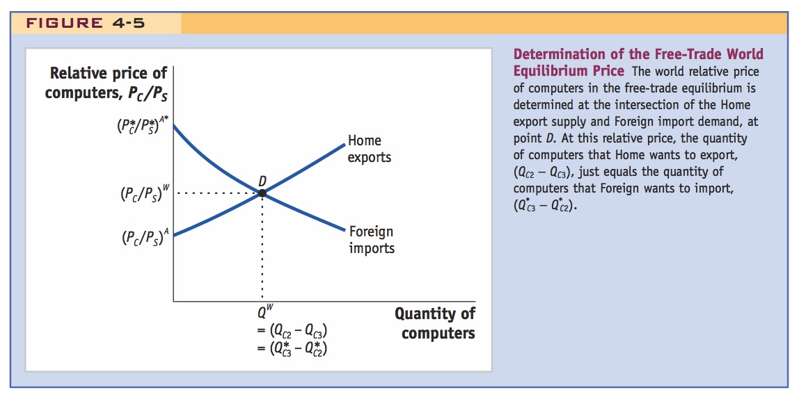
Equilibrium Price with Free Trade As we see in Figure 4-5, the equilibrium relative price of computers with free trade is determined by the intersection of the Home export supply and Foreign import demand curves, at point D (the same as point D in Figure 4-3 or D* in Figure 4-4). At that relative price, the quantity of computers that the Home country wants to export equals the quantity of computers that Foreign wants to import; that is, (Q_C₂ − Q_C₃) = (). Because exports equal imports, there is no reason for the relative price to change and so this is a free-trade equilibrium. Another way to see the equilibrium graphically is to notice that in panel (a) of Figures 4-3 and 4-4, the trade triangles of the two countries are identical in size—the quantity of computers one country wants to sell is the same as the quantity the other country wants to buy.

Pattern of Trade Using the free-trade equilibrium, we have determined the pattern of trade between the two countries. Home exports computers, the good that uses intensively the factor of production (capital) found in abundance at Home. Foreign exports shoes, the good that uses intensively the factor of production (labor) found in abundance there. This important result is called the Heckscher-Ohlin theorem.

Heckscher-Ohlin Theorem: With two goods and two factors, each country will export the good that uses intensively the factor of production it has in abundance and will import the other good.

It is useful to review the assumptions we made at the beginning of the chapter to see how they lead to the Heckscher-Ohlin theorem.

Assumption 1: Labor and capital flow freely between the industries.
Assumption 2: The production of shoes is labor-intensive as compared with computer production, which is capital-intensive.
Assumption 3: The amounts of labor and capital found in the two countries differ, with Foreign abundant in labor and Home abundant in capital.
Assumption 4: There is free international trade in goods.
Assumption 5: The technologies for producing shoes and computers are the same across countries.
Assumption 6: Tastes are the same across countries.

You've just derived all this in detail, but asking them to think through the importance of each assumption and working through the logic will help to make it all fit together.

Assumptions 1 to 3 allowed us to draw the PPFs of the two countries as illustrated in Figure 4-2, and in conjunction with assumptions 5 and 6, they allowed us to determine that the no-trade relative price of computers in Home was lower than the no-trade relative price of computers in Foreign; that is, (P_C/P_S)^A was less than . This key result enabled us to determine the starting points for the Home export supply curve for computers (point A) and the Foreign import demand curve for computers (point A*) in panel (b) of Figures 4-3 and 4-4. Using those starting points, we put together the upward-sloping Home export supply curve and downward-sloping Foreign import demand curve. We see from Figure 4-5 that the relative price of computers in the free-trade equilibrium lies between the no-trade relative prices (which confirms the expectation we had when drawing Figures 4-3 and 4-4).

Therefore, when Home opens to trade, its relative price of computers rises from the no-trade equilibrium relative price (P_C/P_S)^A, to the free-trade equilibrium price (P_C/P_S)^W, giving Home firms an incentive to export computers. That is, higher prices give Home an incentive to produce more computers than it wants to consume, and export the difference. Similarly, when Foreign opens to trade, its relative price of computers falls from the no-trade equilibrium price , to the trade equilibrium price (P_C/P_S)^W, encouraging Foreign consumers to import computers from Home. That is, lower prices give Foreign an incentive to consume more computers than it wants to produce, importing the difference.

You might think that the Heckscher-Ohlin theorem is somewhat obvious. It makes sense that countries will export goods that are produced easily because the factors of production are found in abundance. It turns out, however, that this prediction does not always work in practice, as we discuss in the next section.