4 Intra-Industry Trade and the Gravity Equation
1. Index of Intra-Industry Trade
An index that measures how much of trade is intra-industry. Examples of industries with a high and low intra-industry trade indices. Intra-industry trade requires product differentiation and similar costs.
2. The Gravity Equation
The gravity equation asserts that countries with larger GDPs tend to trade more with each other.
a. Newton’s Universal Law of Gravitation
Analogy from physics, Newton’s law: Fg = G•M1•M2/d2 The greater the mass of two objects (M1 and M2), or the closer they are (d is distance), the greater the force of gravity Fg between them.
b. The Gravity Equation in Trade
Instead of “mass,” use GDP in the two countries; instead of the force of gravity, use the amount of trade. Formula: Trade = B•GDP1GDP2•distn. Bcaptures things other than GDP that could affect trade; rather than 2 because we don’t know exactly how distance affects trade. So trade increases with size, and decreases with distance. This is consistent with the monopolistic competition model: Larger economies export more because they can produce more varieties, and they import more because their demand is greater.
c. Deriving the Gravity Equation
A country’s (country 1) GDP consists of differentiated products. The demand for these goods by an importing country (country 2) will be greater (1) the greater is its relative size and (2) the closer the distance. Measure relative size by its share of world GDP. Then, 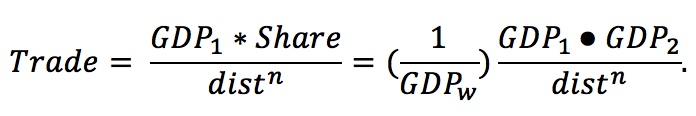 So, B = 1⁄GDPw (and Share = GDP2/GDPw).
In the monopolistic competition model, countries both import and export different varieties of differentiated goods. This result differs from the Ricardian and Heckscher-Ohlin models that we studied in Chapters 2 and 4: in those models, countries either export or import a good but do not export and import the same good simultaneously. Under monopolistic competition, countries will specialize in producing different varieties of a differentiated good and will trade those varieties back and forth. As we saw from the example of golf clubs at the beginning of the chapter, this is a common trade pattern that we call intra-industry trade.
188
Index of Intra-Industry Trade
To develop the idea of intra-industry trade, consider the U.S. imports and exports of the goods shown in Table 6-4. In 2012 the United States imported $1,731 million in vaccines and exported $2,514 million. When the amounts of imports and exports are similar for a good, as they are for vaccines, it is an indication that much of the trade in that good is intra-industry trade. The index of intra-industry trade tells us what proportion of trade in each product involves both imports and exports: a high index (up to 100%) indicates that an equal amount of the good is imported and exported, whereas a low index (0%) indicates that the good is either imported or exported but not both.
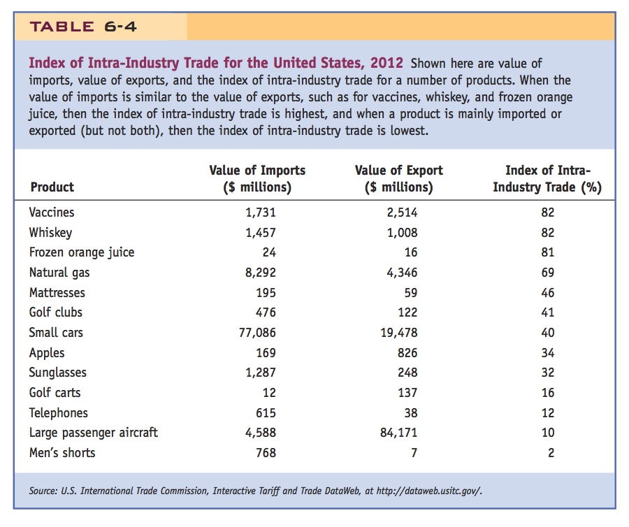
The formula for the index of intra-industry trade is

For vaccines, the minimum of imports and exports is $1,731 million, and the average of imports and exports is  (1,731 + 2,514) = $2,123 million. So
  = 82% of the U.S. trade in vaccines is intra-industry trade; that is, it involves both exporting and importing of vaccines.
In Table 6-4, we show some other examples of intra-industry trade in other products for the United States. In addition to vaccines, products such as whiskey and frozen orange juice have a high index of intra-industry trade. These are all examples of highly differentiated products: for vaccines and whiskey, each exporting country sells products that are different from those of other exporting countries, including the United States. Even frozen orange juice is a differentiated product, once we realize that it is imported and exported in different months of the year. So it is not surprising that we both export and import these products. On the other hand, products such as men’s shorts, large passenger aircraft, telephones, and golf carts have a low index of intra-industry trade. These goods are either mainly imported into the United States (like men’s shorts and telephones) or mainly exported (like large passenger aircraft and golf carts). Even though these goods are still differentiated, we can think of them as being closer to fitting the Ricardian or Heckscher-Ohlin model, in which trade is determined by comparative advantage, such as having lower relative costs in one country because of technology or resource abundance. To obtain a high index of intra-industry trade, it is necessary for the good to be differentiated and for costs to be similar in the Home and Foreign countries, leading to both imports and exports.
Students sometimes ask which explanation (Ricardo, HO, economies of scale) is "right." This is a nice place to make the point that it "all depends" upon what types of goods we are talking about.
189
The Gravity Equation
The index of intra-industry trade measures the degree of intra-industry trade for a product but does not tell us anything about the total amount of trade. To explain the value of trade, we need a different equation, called the “gravity equation.” This equation was given its name by a Dutch economist and Nobel laureate, Jan Tinbergen. Tinbergen was trained in physics, so he thought about the trade between countries as similar to the force of gravity between objects: Newton’s universal law of gravitation states that objects with larger mass, or that are closer to each other, have a greater gravitational pull between them. Tinbergen’s gravity equation for trade states that countries with larger GDPs, or that are closer to each other, have more trade between them. Both these equations can be explained simply—even if you have never studied physics, you will be able to grasp their meanings. The point is that just as the force of gravity is strongest between two large objects, the monopolistic competition model predicts that large countries (as measured by their GDP) should trade the most with one another. There is much empirical evidence to support this prediction, as we will show.
Newton’s Universal Law of Gravitation Suppose that two objects each have mass M1 and M2 and are located distance d apart. According to Newton’s universal law of gravitation, the force of gravity Fg between these two objects is
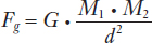
where G is a constant that tells us the magnitude of this relationship. The larger each object is, or the closer they are to each other, the greater is the force of gravity between them.
The Gravity Equation in Trade The equation proposed by Tinbergen to explain trade between countries is similar to Newton’s law of gravity, except that instead of the mass of two objects, we use the GDP of two countries, and instead of predicting the force of gravity, we are predicting the amount of trade between them. The gravity equation in trade is
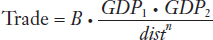
where Trade is the amount of trade (measured by imports, exports, or their average) between two countries, GDP1 and GDP2 are their gross domestic products, and dist is the distance between them. Notice that we use the exponent n on distance, distn, rather than dist2 as in Newton’s law of gravity, because we are not sure of the precise relationship between distance and trade. The term B in front of the gravity equation is a constant that indicates the relationship between the “gravity term” (i.e., GDP1 · GDP2/distn) and Trade. It can also be interpreted as summarizing the effects of all factors (other than size and distance) that influence the amount of trade between two countries; such factors include tariffs (which would lower the amount of trade and reduce B), sharing a common border (which would increase trade and raise B), and so on.
190
Observe that this is a beautiful implication of the theory.
According to the gravity equation, the larger the countries are (as measured by their GDP), or the closer they are to each other, the greater is the amount of trade between them. This connection among economic size, distance, and trade is an implication of the monopolistic competition model that we have studied in this chapter. The monopolistic competition model implies that larger countries trade the most for two reasons: larger countries export more because they produce more product varieties, and they import more because their demand is higher. Therefore, larger countries trade more in both exports and imports.
Deriving the Gravity Equation To explain more carefully why the gravity equation holds in the monopolistic competition model, we can work through some algebra using the GDPs of the various countries. Start with the GDP of Country 1, GDP1. Each of the goods produced in Country 1 is a differentiated product, so they are different from the varieties produced in other countries. Every other country will demand the goods of Country 1 (because they are different from their home-produced goods), and the amount of their demand will depend on two factors: (1) the relative size of the importing country (larger countries demand more) and (2) the distance between the two countries (being farther away leads to higher transportation costs and less trade).
To measure the relative size of each importing country, we use its share of world GDP. Specifically, we define Country 2’s share of world GDP as Share2 = GDP2/GDPW. To measure the transportation costs involved in trade, we use distance raised to a power, or distn. Using these definitions, exports from Country 1 to Country 2 will equal the goods available in Country 1 (GDP1), times the relative size of Country 2 (Share2), divided by the transportation costs between them (distn), so that
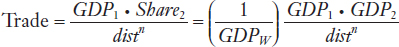
This equation for the trade between Countries 1 and 2 looks similar to the gravity equation, especially if we think of the term (1/GDPW) as the constant term B. We see from this equation that the trade between two countries will be proportional to their relative sizes, measured by the product of their GDPs (the greater the size of the countries, the larger is trade), and inversely proportional to the distance between them (the smaller the distance, the larger is trade). The following application explores how well the gravity equation works in practice.
Using n = 1.25, the gravity equation fits the data between the states in the U.S. and Canadian provinces very well, as well as between provinces in Canada. However, trade across borders is less than trade within borders because of barrier effects.
The Gravity Equation for Canada and the United States
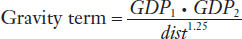
We can apply the gravity equation to trade between any pair of countries, or even to trade between the provinces or states of one country and another. Panel (a) of Figure 6-9 shows data collected on the value of trade between Canadian provinces and U.S. states in 1993. On the horizontal axis, we show the gravity term:
191
where GDP1 is the gross domestic product of a U.S. state (in billions of U.S. dollars), GDP2 is the gross domestic product of a Canadian province (in billions of U.S. dollars), and dist is the distance between them (in miles). We use the exponent 1.25 on the distance term because it has been shown in other research studies to describe the relationship between distance and trade value quite well. The horizontal axis is plotted as a logarithmic scale, with values from 0.001 to 100. A higher value along the horizontal axis indicates either a large GDP for the trading province and state or a smaller distance between them.
192
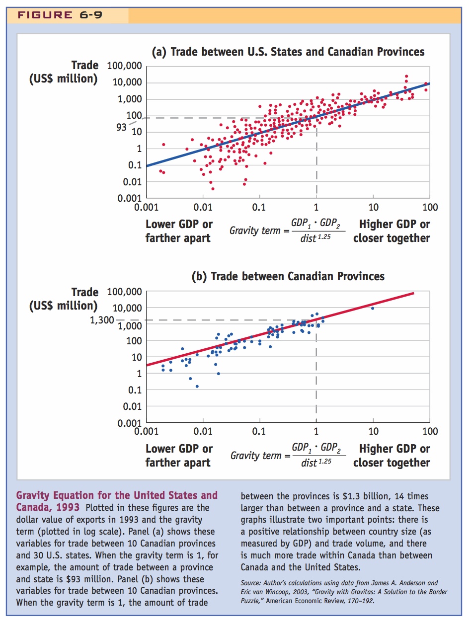
The vertical axis in Figure 6-9 shows the 1993 value of exports (in millions of U.S. dollars) between a Canadian province and U.S. state or between a U.S. state and Canadian province; this is the value of trade for the province–state pair. That axis is also plotted as a logarithmic scale, with values from $0.001 million (or $1,000) to $100,000 million (or $100 billion) in trade. There are 30 states and 10 provinces included in the study, so there are a total of 600 possible trade flows between them (though some of those flows are zero, indicating that no exporting takes place). Each of the points in panel (a) represents the trade flow and gravity term between one state and one province.
We can see from the set of points in panel (a) that states and provinces with a higher gravity term between them (measured on the horizontal axis) also tend to have more trade (measured on the vertical axis). That strong, positive relationship shown by the set of points in panel (a) demonstrates that the gravity equation holds well empirically. Panel (a) also shows the “best fit” straight line through the set of points, which has the following equation:
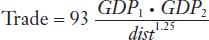
The constant term B = 93 gives the best fit to this gravity equation for Canadian provinces and U.S. states. When the gravity term equals 1, as illustrated in panel (a), then the predicted amount of trade between that state and province is $93 million. The closest example to this point is Alberta and New Jersey. In 1993 there were $94 million in exports from Alberta to New Jersey and they had a gravity term of approximately 1.
Trade Within Canada Because the gravity equation works well at predicting international trade between provinces and states in different countries, it should also work well at predicting trade within a country, or intra-national trade. To explore this idea, panel (b) of Figure 6-9 graphs the value of exports (in millions of U.S. dollars) between any two Canadian provinces, along with the gravity term for those provinces. The scale of the axes in panel (b) is the same as in panel (a). From panel (b), we again see that there is a strong, positive relationship between the gravity term between two provinces (measured on the horizontal axis) and their trade (measured on the vertical axis). The “best fit” straight line through the set of points has the following equation:
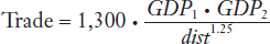
That is, the constant term B = 1,300 gives the best fit to this gravity equation for Canadian provinces. When the gravity term equals 1, as illustrated in panel (b), then the predicted amount of trade between two provinces is $1,300 million, or $1.3 billion. The closest example to this combination is between British Columbia and Alberta: in 1993 their gravity term was approximately 1.3 and British Columbia exported $1.4 billion of goods to Alberta.
Comparing the gravity equation for international trade between Canada and the United States with the gravity equation for intra-national trade in Canada, the constant term for Canadian trade is much bigger—1,300 as compared with 93. Taking the ratio of these two constant terms (1,300/93 = 14), we find that on average there is 14 times more trade within Canada than occurs across the border! That number is even higher if we consider an earlier year, 1988, just before Canada and the United States signed the Canada–U.S. Free Trade Agreement in 1989. In 1988 intra-national trade within Canada was 22 times higher than international trade between Canada and the United States.14 Even though that ratio fell from 1988 to 1993 because of the free-trade agreement between Canada and the United States, it is still remarkable that there is so much more trade within Canada than across the border, or more generally, so much more intra-national than international trade.
193
The finding that trade across borders is less than trade within countries reflects all the barriers to trade that occur between countries. Factors that make it easier or more difficult to trade goods between countries are often called border effects, and they include the following:
- Taxes imposed when imported goods enter into a country, tariffs
- Limits on the number of items allowed to cross the border, quotas
- Other administrative rules and regulations affecting trade, including the time required for goods to clear customs
- Geographic factors such as whether the countries share a border
- Cultural factors such as whether the countries have a common language that might make trade easier
In the gravity equation, all the factors that influence the amount of trade are reflected in the constant B. As we have seen, the value of this constant differs for trade within a country versus trade between countries. In later chapters, we explore in detail the consequences of tariffs, quotas, and other barriers to trade. The lesson from the gravity equation is that such barriers to trade can potentially have a large impact on the amount of international trade as compared with intra-national trade.
All of which make it odd that the U.S./Canadian border should have much effect at all. But you might elaborate upon this by mentioning the large deviations from LOOP caused by the U.S./Canadian border too.